Reader TTS

ABSTRACT In the Southern Ocean, large-scale phytoplankton blooms occur in open water and the sea-ice zone (SIZ). These blooms have a range of fates including physical advection, downward

carbon export, or grazing. Here, we determine the magnitude, timing and spatial trends of the biogeochemical (export) and ecological (foodwebs) fates of phytoplankton, based on seven

BGC-Argo floats spanning three years across the SIZ. We calculate loss terms using the production of chlorophyll—based on nitrate depletion—compared with measured chlorophyll. Export losses

are estimated using conspicuous chlorophyll pulses at depth. By subtracting export losses, we calculate grazing-mediated losses. Herbivory accounts for ~90% of the annually-averaged losses

(169 mg C m−2 d−1), and phytodetritus POC export comprises ~10%. Furthermore, export and grazing losses each exhibit distinctive seasonality captured by all floats spanning 60°S to 69°S.

These similar trends reveal widespread patterns in phytoplankton fate throughout the Southern Ocean SIZ. SIMILAR CONTENT BEING VIEWED BY OTHERS WIDESPREAD CHANGES IN SOUTHERN OCEAN

PHYTOPLANKTON BLOOMS LINKED TO CLIMATE DRIVERS Article Open access 28 August 2023 ATLAS OF PHYTOPLANKTON PHENOLOGY INDICES IN SELECTED EASTERN MEDITERRANEAN MARINE ECOSYSTEMS Article Open

access 30 April 2024 LARGE DIATOM BLOOM OFF THE ANTARCTIC PENINSULA DURING COOL CONDITIONS ASSOCIATED WITH THE 2015/2016 EL NIÑO Article Open access 09 December 2021 INTRODUCTION

Phytoplankton in the Southern Ocean produce new particles, driving the biological carbon pump that plays a disproportionately important role in global climate on a range of time scales1,2.

Phytoplankton also supply energy to support Antarctic krill, the most abundant animal on the planet by mass3, and the link to apex predators. In the Southern Ocean, satellite remote-sensing

reveals that the sea-ice zone (SIZ) accounts for ~15% of the basin-scale primary production4. The productivity of the SIZ also plays a strong role in setting the magnitude of the downward

particle flux, via the rapid sinking of sea-ice edge blooms5, and sea ice is a critical habitat for overwintering krill6. At decadal time scales, the fate of phytoplankton is changing in the

SIZ due to environmental forcing7,8. A climate-change related reduction in sea-ice cover could have dramatic consequences for biogeochemistry and ecology if the fate of phytoplankton is

altered9,10,11. Biogeochemical (BGC) Argo floats are a relatively recent technological development that provide vertical profiles of chlorophyll (chl) and particles (both proxies for

phytoplankton biomass), along with temperature, salinity, pH, dissolved oxygen and nitrate concentration12. These observations are particularly valuable for polar oceans, where fewer in situ

observations have been made. Floats can also sense the water column during the polar night and under the sea ice where satellites cannot view13, providing unique time series of

phytoplankton growth and particulate organic carbon (POC) export dynamics14. Chl concentration is routinely used to derive primary production remotely from satellite15,16 but little effort

has focused on the logical next step—assessing the fate of phytoplankton blooms17. Information on the fate of phytoplankton is valuable as it helps to partition losses due to physical

(advection), biogeochemical (export) and ecological (grazing and mortality as part of pelagic foodwebs) processes18. The objective of this study is to assess patterns in the biogeochemical

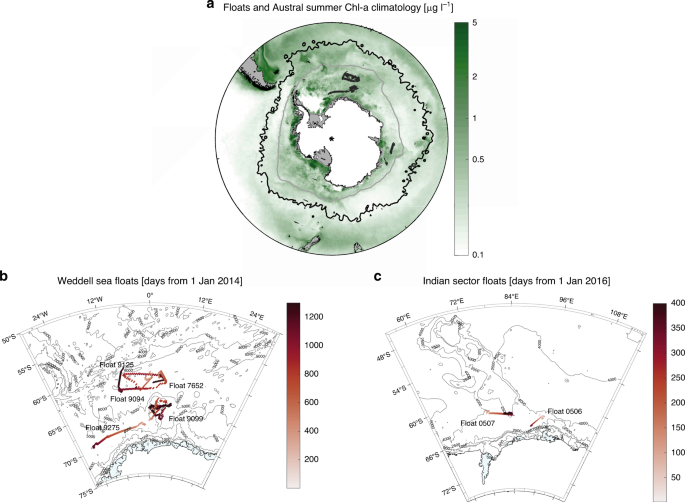
and ecological fates of primary producers as revealed through careful analysis of BGC-Argo multi-sensor datasets for seven widely distributed SOCCOM (Southern Ocean Carbon and Climate

Observations and Modelling) floats that drifted across the SIZ of the Weddell Sea and the Indian Ocean sector of the Southern Ocean, between 60° S and 69° (see “Methods” and Fig. 1). Our

findings on the distinctive seasonality of the fate of phytoplankton represent a step forward in our understanding of drivers of biogeochemistry and ecology at high latitudes, where few

continuous time series exist in open water19 or in the dynamic SIZ20. RESULTS CALCULATING CHLOROPHYLL PRODUCTION AND LOSSES The development of an approach to tease apart the fate of chl

relies first on calculating its potential production (i.e., de novo synthesis), comparing this with measured chl, then assessing the cumulative losses due to advection, vertical export,

grazing and mortality18. The first step relies on knowledge that phytoplankton photosynthesis produces chl via the consumption of NO3− at known rates. For phytoplankton and sea-ice algae the

ratio of chl synthesis to nitrate uptake (chl:N) varies between 0.34 and 2.47 µg chl:µmol N as reported in field studies and laboratory cultures across sites ranging from polar to tropical

waters21,22,23,24,25,26 (a sensitivity analysis of the method to the chl:N ratio is presented in the “Methods”). A recent biogeochemical budget for the Amundsen Sea Polynya23 provides a very

detailed, multi-station time series of nitrate depletion and concurrent accumulation of chl during a rapidly evolving bloom (average ratio 1.75 ± 0.4 µg chl:µmol N) from a polynya analogous

to the SIZ we studied using BGC-Argo. Thus, from nitrate drawdown and this reference value of chl:N = 1.75 µg chl:µmol N, we calculate potential chl synthesis without any losses, so long as

ocean physics enables a comparison of consecutive nitrate profiles derived from BGC-Argo. We were able to rule out advection as a loss term for chl and nitrate, because changes in physical

properties were at least an order of magnitude smaller than published criteria for consideration of contiguous profiles (see “Methods” and Ref. 27). Each winter, nutrient inventories (here

nitrate, NO3−) are reset in the upper ocean by deep vertical mixing. That is, the concentration over the upper few hundred metres becomes almost uniform and equivalent to the deep

concentration. Using a chl:_N_ ratio of 1.75 µg chl:µmol N for our reference value and the salinity-normalized NO3− drawdown relative to the closest winter NO3− profile (ΔNO3−, Fig. 2a), we

can calculate the concentration of chl (chl*) that should be present in the absence of losses (Fig. 2b): $${\mathrm{chl}}^ \ast = 1.75 \times \Delta {\mathrm{NO}}_3^ -.$$ (1) Chl

concentration is measured by a calibrated in vivo fluorescence sensor on the BGC-Argo float, corrected for nonphotochemical quenching28 and assumed to represent biomass12 after losses:

$${\mathrm{chl}} = {\mathrm{chl}}^\ast - {\mathrm{total}}\;{\mathrm{losses}}.$$ (2) The difference between chl* and the observed chl (Fig. 2c) represents a proxy for the total losses of

phytoplankton biomass (Fig. 2d): $${\mathrm{total}}\;{\mathrm{losses}} = {\mathrm{chl}}^\ast - {\mathrm{chl}}.$$ (3) Total losses can be partitioned into local and distal losses, where

distal losses are downward export, because we eliminated horizontal advection: $${\mathrm{total}}\;{\mathrm{losses}} = {\mathrm{local}}\;{\mathrm{losses}} + {\mathrm{export}}.$$ (4) The

downward export of chl as phytodetritus (i.e., phytoplankton aggregates and senescent cells29) is conspicuous in BGC-Argo profiles below the export depth (i.e., the deeper of either the

surface mixed layer, ML, or the euphotic zone depth, Zeu; see “Methods”) where it corresponds to higher (i.e., excess) chl concentrations than that expected from the negligible observed NO3−

drawdown at these depths (Fig. 2e). The export of phytodetritus is first observed below the export depth in early spring and is coincident with observations of POC export from the BGC-Argo

backscattering sensors (Fig. 2f). This early export of phytodetritus and POC, following the stratification of the water column, was consistently observed among all seven floats

(Supplementary Figs. 1 and 2), in agreement with previous studies that showed that shallow transient stratification close to spring led to more favourable conditions for primary production

and carbon export in the Southern Ocean14. Losses of chl due to downward export were calculated using conspicuous excess chl pulses at depth (between the export depth and 175 m, the deepest

winter mixed layer estimated from all seven floats, see “Methods”). After calculating phytodetritus downward export, local losses were calculated as the difference between total losses

(between the surface and 175 m) and downward export (between the export depth and 175 m): $${\mathrm{local}}\;{\mathrm{losses}} = {\mathrm{total}}\;{\mathrm{losses}} - {\mathrm{export}}.$$

(5) Local losses of chl can be due to physiological and ecological processes: mortality and grazing, respectively (Fig. 2d). Mortality (defined here as intrinsically driven mortality in

response to environmental stresses such as nutrient starvation30) was calculated from published oceanic rates used in modelling31 and subtracted from local losses, leaving grazing. We have

included viral lysis in the grazing term in these calculations, due to the dearth of knowledge available to tease grazing and lysis apart for the SIZ. $${\mathrm{grazing}} =

{\mathrm{local}}\;{\mathrm{losses}}-{\mathrm{mortality}}.$$ (6) Finally, the phytoplankton biomass accumulation was calculated from positive changes in integrated observed chl15. Chl losses

and biomass accumulation were converted to carbon units to assess the contribution of phytodetritus POC export to downward POC export (see “Methods”). This approach is described

schematically in Fig. 3. Following previous work that estimated POC export from sensors mounted on lagrangian floats32,33, we estimate POC export from the POC increment below the export

depth and down to 175 m between consecutive profiles. The downward POC export includes phytodetritus and particles transformed by the foodweb such as faecal pellets34 (see “Methods”), and is

calculated over the same depth stratum as phytodetritus POC export. Other studies (Dall’Olmo et al.33 and Briggs et al.35) measured the sinking of small particles through the mesopelagic

layer using backscattering sensors mounted on BGC-Argo floats. Using this approach, Briggs et al.35 highlighted that particulate fragmentation was responsible for 49 ± 22% of the observed

flux loss between 100 and 1000 m. Our method, using BGC-Argo sensors to estimate carbon export, can not account for the bacterial remineralization of particulates into dissolved organic

carbon (DOC). In addition, large backscattering spikes might be caused by the presence of zooplankton as shown by Bishop and Wood36, which would lead us to overestimate POC export.

BIOGEOCHEMICAL LOSSES OF CHLOROPHYLL Phytodetritus POC export takes place from October to April, and is at its highest from December to March (Fig. 4a). The maximum measured export of

phytodetritus POC was 413 mg C m−2 d−1 early in the production season, on December 28, 2016, by float #9275 in the south of the Weddell Sea (Supplementary Fig. 1). Maximum downward POC

export was 600 mg C m−2 d−1 measured on February 2, 2016, by float #0506 (Fig. 4b), and was in the range of previous maximum estimates from the open Southern Ocean to the SIZ (1090 mg C m−2 

d−1; Ref. 37). Pooling the seven BGC-Argo float datasets we studied, POC export follows phytodetritus POC export through the phytoplankton production season, and is highest from December to

March (Fig. 4b). However, compared with phytodetritus POC export, POC export starts a little later, in November compared with October. Our analysis provides seasonal trends in the

contribution of phytodetritus to downward POC export. Where POC and phytodetritus POC export coincide, we find that the export of phytodetritus accounts for 24% on average of the total

export of POC (Fig. 4c and Supplementary Fig. 3). However, the annually averaged POC and phytodetritus POC export calculated for all the BGC-Argo floats are 79 and 19 mg C m−2 d−1,

respectively, which considers all seasons. Hence the contribution of phytodetritus over the annual cycle is ~19%. This contribution is variable during the winter months (with few estimates

from May to October) but consistent throughout the productive season, although slightly higher at the beginning of the production season (November–December) than at the end (January–March,

Fig. 4c). At the onset of the production season, the contribution of grazers to POC export via faecal pellets or vertical migration is expected to be lower as grazers may still be

overwintering at depth38. ECOLOGICAL FATE OF PHYTOPLANKTON After calculating the direct export of chl as phytodetritus, grazing is determined by difference since physical losses are

negligible. Chl losses are mainly observed between the surface and the export depth consistent with herbivory (Fig. 2d). However, to be consistent with our phytodetritus POC export

calculations, losses due to grazing were integrated from the surface to 175 m depth. The maximum grazing rate was 965 mg C m−2 d−1, measured on January 13, 2015 by float #7652 in the Weddell

Sea (Fig. 4d). Previously, modelling studies39 have calculated upper bound grazing rates of 400–700 mg C d−1 for the coastal and open Southern Ocean. Pooling all BGC-Argo floats considered

here, we find annually averaged grazing rates of 169 mg C m−2 d−1 (Fig. 4d). This analysis is the first basin scale, observational estimate of grazing throughout the SIZ of the Southern

Ocean. In comparison, we observe relatively little accumulation of phytoplankton in the SIZ (Fig. 4f). The annually averaged phytoplankton biomass accumulation calculated for all the

BGC-Argo floats was 40 mg C m−2 d−1. The maximum phytoplankton biomass accumulation was 543 mg C m−2 d−1, measured by float #9099 in the Weddell Sea on January 3, 2016. Pooling all float

datasets, we can also derive the seasonal influence of grazing on chl. An increase in herbivory is observed from October to December, while higher grazing pressure is fairly constant

throughout the second part of the growing season, January–June, 3 months after the main downward export events (Fig. 4d). Grazing decreases during winter (July–October) but does not fall to

zero, consistent with observations that krill and other zooplankton feed throughout winter for their survival40. For all float datasets, where phytodetritus POC export events and grazing

rates are coincident, grazing contributes 83% of total chl losses, on average. However, a comparison of the annually averaged grazing rates (169 mg C m−2 d−1) to the annually averaged

phytodetritus POC export (19 mg C m−2 d−1) for all float datasets takes the contribution of grazing to total chl losses to ~90%. The remaining 10% is downward export of phytodetritus. This

trend is consistent throughout the year for all floats, except in November, at the beginning of the production season, when the impact of grazing is slightly lower (Fig. 4e). This is

consistent with the higher contribution of phytodetritus to total export at the beginning of the production season. Furthermore, the dominance of grazing throughout most of the year confirms

the primary role of zooplankton in controlling the fate of phytoplankton in the Southern Ocean41,42. SENSITIVITY OF THE METHOD TO THE CHL:N RATIO To account for the potential variability in

the chl:N ratio, we ran a detailed sensitivity analysis of our approach to the chl:_N_ ratio (see Methods). The results of the sensitivity analysis for all floats is given in Table 1. We

find that the average export of phytodetritus for all floats is 22 ± 3, 19 ± 3 and 18 ± 3 mg C d−1 for chl:N ratios of 1.25, 1.75 and 2.5 µg chl:µmol N, respectively. Similarly, average

grazing for all floats is 126 ± 7, 169 ± 10 and 233 ± 13 mg C d−1 for chl:N ratios of 1.25, 1.75 and 2.5 µg chl:µmol N, respectively. Thus, the contribution of grazing to total chl losses is

85, 90 and 93% for varying chl:N ratios of 1.25, 1.75 and 2.5 µg chl:µmol N, confirming the prevalence of grazing on chl losses in the SIZ of the Southern Ocean. DISCUSSION The seven floats

we studied span the Weddell Sea and the Indian Ocean sector of the SIZ between 60 and 69° S (Fig. 1). Despite this wide range of locales sampled, we find no statistically significant

differences in the magnitude of phytodetritus POC export, POC downward export and grazing across the SIZ (Fig. 5). The only departure from this prevalent trend is higher phytodetritus POC

export at 69° S (Fig. 5a). This event may be due to a combination of higher rates of phytoplankton biomass accumulation compared with the rest of the SIZ (Fig. 5f) but a grazing loss term

that is comparable to other latitudes (Fig. 5d). We also find no statistically significant differences in the magnitude of phytodetritus POC export, POC export and grazing between sampling

years (2015–2017, Supplementary Fig. 4), between floats (Supplementary Fig. 5), and between the SIZ areas studied: the Weddell Sea and Prydz Bay (Supplementary Fig. 6). This evidence of

widespread and consistent seasonality in the phytodetritus and herbivory loss terms is striking but has a number of plausible explanations. First, since this study is focused in the Southern

Ocean SIZ, the major phytoplankton grazers are likely to be Antarctic krill, _Euphausia superba_43. The spatially uniform nature of the fate of blooms is inconsistent with the known patchy

distribution of krill3. Hence, the uniformity suggests that on longer time scales the krill patchiness may be averaged out, by the lateral advection of krill patches44. Second, this study

focuses on BGC-Argo floats that had trajectories within the latter two of the three major krill development areas which are: the Scotia Sea and Antarctic Peninsula; the eastern Weddell and

Lazarev Seas; and the north of Prydz bay and the Kerguelen Plateau45. The constancy of chl loss terms due to herbivory across the SIZ could be linked to the ubiquitous grazing pressure of

krill in these areas, which dominates losses46. Analysis of floats from outside of known krill development areas could confirm, or not, the extent to which phytoplankton losses are uniform

across the SIZ. Third, our data may alternatively reflect that copepod herbivory dominates where krill herbivory is absent47,48. The early season dominance of phytodetritus POC export as a

major loss term is probably due to the similarity in the drivers of primary productivity across the SIZ, where sea-ice melt in spring typically releases large amounts of dissolved and

particulate iron to surface waters49. This nutrient delivery, coupled with a shallow meltwater- and temperature-driven mixed layer, fosters the sea-ice edge blooms in which phytoplankton

growth is decoupled from grazing50. The inaccessibility, over much of the annual cycle, of both the open water regions and the SIZ of the Southern Ocean has resulted in a limited vison of

how the regional biogeochemistry and ecology function, with little known about how they interact. Satellite oceanography, using a range of sensors, has led to major advances in understanding

the seasonality of phytoplankton blooms and how it can be linked to other remotely sensed environmental drivers such as satellite-derived sea-ice extent and upper ocean temperature51.

However, satellite oceanography has for some sensors been hindered by the cloudiness that characterized much of the Southern Ocean. Our findings illustrate how profiling BGC-Argo floats can

complement other platforms and potentially launch significant advances in our understanding in the same way that satellite ocean colour has since the 1990s. Given the complexity of assessing

the status of this ecosystem and the carbon cycle, our approach enables quantification of the fates of phytoplankton in the SIZ on a short time scale (10 days) throughout the annual cycle,

and moreover to map their seasonality across a range of diverse locales. In comparison, other estimates of net community production based on export or nitrate drawdown relative to winter27,

are on a seasonal to annual time scale. Some of the most recent BGC-Argo floats are equipped with Underwater Vision Profilers (UVP6) which will allow counting organisms from bacteria to

zooplankton52. The ability to discern the fate of SIZ phytoplankton is essential for understanding the current magnitude of, and future trends in the high-latitude biological pump and

ecosystems. METHODS THE SEA-ICE ZONE We studied seven SOCCOM floats that drifted across the SIZ of the Weddell Sea and the Indian Ocean sector of the Southern Ocean, between 60 and 69° S

(Fig. 1a). The Weddell Sea is a large cyclonic gyre. Northeast of the Weddell Gyre, the Southwest Indian Ridge was identified as a major topographic feature where circumpolar deep water

(CDW) travels southward through the Antarctic Circumpolar Current (ACC)53. South of the ACC, CDW is upwelled to the surface through wind-driven divergence and is modified on its path through

the Weddell Gyre (then called Warm Deep Water, WDW54). Five BGC-Argo floats drifted across the open waters of the eastern Weddell Gyre (Fig. 1b), a region that was identified as a major

carbon sink due to strong primary production55. The Kerguelen Plateau is a major obstacle on the eastward flow of the ACC. The bulk of the ACC passes north of the Kerguelen Plateau, while

the remainder passes through the Fawn Trough (at ~56° S) or through the Princess Elizabeth Trough (at ~64° S), south of the Banzare Bank56 (Fig. 1c). Two BGC-Argo floats drifted in the

highly productive SIZ, south of the Banzare bank57. The temperature and salinity sections of all seven floats are typical of ice-covered regions (Supplementary Figs. 7 and 8), with increases

in mixed layer salinity under sea ice during winter and the classic thermal signature of winter water colder than −1 °C at 100 m deep14. The SOCCOM floats we studied park and drift at 1000 

m, and descend to 2000 m before returning to the surface every 10 days. CRITERIA NECESSARY TO DEVELOP THE ALGORITHM Changes in water mass properties in the 10 days window between profiles

can rule out the comparison of sequential float profiles. Hence, we first assessed advection between consecutive profiles via a careful analysis of physical properties. Horizontal loss terms

can be regarded as not significant if changes in physical properties are negligible. To successfully infer net community production from BGC-Argo floats in the Southern Ocean, Johnson et

al.27 imposed three criteria: (1) that the salinity at 500 m did not change by more than 0.05 between two consecutive profiles, (2) that the latitude did not change by more than 5.5° and (3)

that the longitude did not change by more than 8°. For all the BGC-Argo floats studied here, we found average (maximum) changes of 0.0013 (0.017) for salinity at 500 m, 0.07° (0.45°) for

latitude, and 0.22° (1.1°) for longitude between two consecutive profiles. That is, the changes we observed were at least an order of magnitude smaller than the Johnson et al. criteria.

Water column properties in the SIZ are, therefore, highly stable between successive CTD profiles, which makes it reasonable to compare the temporal evolution of biogeochemical properties and

ignore horizontal and vertical advection as influential loss terms for chl. That is, we consider consecutive profiles as contiguous. Furthermore, we suggest that this method can be

generalized to other oceanic regions as long as the changes in physical properties between consecutive profiles are minimal. In addition, to estimate NO3− drawdown, we used the

salinity-normalized NO3− profile to correct for dilution and concentration effects linked to sea-ice melt and formation in the SIZ. EXPORT DEPTH AND HORIZON Following Dall’Olmo et al.33, the

export depth is taken as the deeper of either the surface mixed layer (ML, defined from Ref. 58 as the depth at which density increased by 0.01 kg m−3 compared with density at the surface)

or the euphotic zone depth (Zeu, defined by Ref. 59 as the 2% light level and derived from sea surface chl concentration in Antarctic waters) when solar irradiance reaches the ocean surface

(i.e., not during the polar night) as determined by year day and latitude. We acknowledge that other open water studies have used the critical depth rather than the euphotic zone depth as

the upper limit below which to calculate downward export14. However, near the ice edge where the coverage of satellite-derived irradiance data is poor, we find that the euphotic zone

reflects more accurately the depth over which particles may be created. In contrast, the critical depth may be a more powerful metric in open waters as previously shown by Bishop and Wood14.

We chose 175 m (the deepest winter mixed layer estimated from all seven floats) as the depth horizon to calculate export as recent studies demonstrate that the depth of the mixed layer in

winter constrains downward export60. For example, a proportion of the organic matter that is exported below the export depth during the stratified summer months can be ventilated by deep

winter mixing. CONFIRMATION OF DEEP EXCESS CHLOROPHYLL AS PHYTODETRITUS A rationale is presented here for interpreting subsurface excess in chl as phytodetritus (such as aggregated senescent

cells) sinking below the export depth. A few studies showed that diatoms may still be viable after ingestion and excretion by krill61, which could cast uncertainty on our assumption of

observations of phytodetritus below the export depth. However, in the Indian sector of the Southern Ocean, in proximity to Crozet Island and the Kerguelen plateau, widely observed

backscattering and fluorescence excess—that are conspicuous in the profiles below the export depth—were attributed to either faecal pellets or phytodetritus29. The authors argued that the

senescence of phytoplankton does not alter the phytol chain of chl a, which leaves the fluorescence of the prophyrin ring intact. In contrast, zooplankton grazing removes the magnesium ions

from chl a, which results in the accumulation of phaeopigments in faecal pellets. Therefore, we are confident that the positive chl anomalies we observed below the export depth were mainly

composed of phytodetritus. GRAZING RATES ESTIMATES Instantaneous grazing rates can be calculated from the profile-to-profile increments in local losses of chl. First, local losses are

calculated as the difference between total chl losses and the export of phytodetritus below the export depth, that is, phytodetritus POC export (Eq. (5)). Phytoplankton mortality between the

surface and the export depth31 is then subtracted from local losses to leave grazing (Eq. (6)). To constrain this calculation, we further impose three criteria: (1) we only consider

positive changes in local losses. Negative local losses would be caused by the input of nitrate between the surface and the export depth and yield negative grazing rates; (2) we only

subtract positive changes in phytodetritus between the export depth and 175 m, because negative changes would represent export below 175 m and artificially increase grazing rates, and (3) we

only calculate grazing rates when increments in local losses are higher than increments in phytodetritus below the export depth, as the contrary would yield negative grazing rates. The

above-mentioned conditions reduce the number of grazing estimates, but they allow us to constrain grazing rates as close to reality as possible. A reasonable number of grazing estimates (_N_

 = 219) can be obtained via this method. The production of faecal pellets by grazers is where carbon export and foodwebs interact34. Grazing will result in the destruction of chl and the

repackaging of phytoplankton cells into aggregates or faecal pellets. To avoid double accounting of these chl losses, we made a simple distinction between the direct export of phytodetritus

and grazing. CHLOROPHYLL TO CARBON CONVERSION We used three conversion factors to convert chl losses and biomass accumulation to carbon: (1) a lower bound of 20 µg C/µg chl62 to constrain

the minimum downward POC export associated with phytodetritus under saturating light and high nutrient supply, (2) a robust method to derive phytoplankton carbon from chl63,64 (referred to

hereafter as T17 for Thomalla et al.64); and (3) the average POC:chl ratio (in µg C/µg chl) measured in the ML for each separate float (ML POC:chl ratios for all the BGC-Argo floats studied

are shown in Supplementary Fig. 9). We used approach 2 from T17 for our reference value, since it was specifically derived from multiple Southern Ocean glider transects64. This yielded

POC:chl ratios consistent with other approaches based on backscattering65, but it does not account for varying POC:chl ratios with environmental conditions. SENSITIVITY OF THE METHOD TO THE

CHL:N RATIO We tested the sensitivity of the calculated maximum chl concentration to chl:N ratios ranging from 0.5 to 2.5 µg chl:µmol N (Supplementary Fig. 10). First, we found that a lower

bound of 1.25 µg chl:µmol N was appropriate for our calculations, since below this limit, the estimated synthesized chl is consistently lower than the observed chl for 100 days at the

beginning of the production season (days 300–400 in Supplementary Fig. 10a–c). This finding was consistent between all seven of the floats we studied. Furthermore, we chose 2.5 µg chl:µmol N

as a reasonable upper bound for our sensitivity analysis given that it was among the highest reported chl:N values reported in field studies and laboratory cultures across sites ranging

from polar to tropical waters21,22,23,24,25. Next we selected an intermediate chl:N ratio of 1.75 µg chl:µmol N as our reference value. This selection was supported since it is the average

chl:N ratio (1.75 ± 0.4 µg chl:µmol N) observed in the recent detailed Amundsen Sea Polynya (spanning 72.5–74° S)23, across a primary production gradient of integrated dissolved inorganic

nitrogen drawdown (ΔDIN) of 27–740 mmol N m−2 and integrated chl from 74 to 828 mg m−2 (Supplementary Table 1). This detailed, multi-station study is ideal since it presents a time series of

nitrate depletion and concurrent accumulation of chl during a rapidly evolving water column bloom, in the virtual absence of grazers23. There is, however, no such situation when grazers are

completely absent, suggesting that our grazing estimates are possibly underestimated. Furthermore, the Amundsen Sea polynya has the highest primary production rates of all Antarctic

polynyas66. Surrounding the Amundsen Sea polynya, the Dotson and Getz Ice Shelves are among the fastest melting glaciers of Antarctica67, and naturally fertilize the polynya68. Therefore,

the source of dissolved iron is likely different between the Amundsen Sea polynya and the SIZ of the Southern Ocean, with possible effects on the chl:N ratio of phytoplankton. In comparison,

the chl:N ratio reported from the SOFEX-S iron-amended mesoscale bloom in the SIZ (at 66 S) averaged 2.1 µg chl:µmol N, as reported by Coale et al.26 (their Table 1), and was therefore

comparable to the chl:N ratio of 1.75 µg chl:µmol N we chose as reference value. In addition, the in situ chl:N ratio is likely to vary throughout the production season and among

phytoplankton species69. A map of the chl:N ratio (µg chl:µmol N) measured in the Amundsen Sea polynya supports this variability (Supplementary Fig. 10d), with a decreasing ratio eastward,

towards a more developed bloom23. The results of the sensitivity analysis of our approach to the chl:N ratio (from 1.25 to 2.5 µg chl:µmol N) are presented in Table 1 (see “Results”).

REPORTING SUMMARY Further information on research design is available in the Nature Research Reporting Summary linked to this article. DATA AVAILABILITY All SOCCOM data used in the present

paper are available at https://soccom.princeton.edu. REFERENCES * Gottschalk, J. et al. Biological and physical controls in the Southern Ocean on past millennial-scale atmospheric CO2

changes. _Nat. Commun._ 7, 11539 (2016). Article  ADS  CAS  PubMed  PubMed Central  Google Scholar  * Khatiwala, S., Primeau, F. & Hall, T. Reconstruction of the history of anthropogenic

CO2 concentrations in the ocean. _Nature_ 462, 346 (2009). Article  ADS  CAS  PubMed  Google Scholar  * Atkinson, A., Siegel, V., Pakhomov, E. A., Jessopp, M. J. & Loeb, V. A

re-appraisal of the total biomass and annual production of Antarctic krill. _Deep Sea Res. Part I Oceanogr. Res. Pap._ 56, 727–740 (2009). Article  ADS  Google Scholar  * Taylor, M. H.,

Losch, M. & Bracher, A. On the drivers of phytoplankton blooms in the Antarctic marginal ice zone: a modeling approach. _J. Geophys. Res. Oceans_ 118, 63–75 (2013). Article  ADS  Google

Scholar  * Matsuda, O., Ishikawa, S. & Kawaguchi, K. Seasonal variation of particulate organic matter under the antarctic fast ice and its importance to benthic life. in _Antarctic

Ecosystems_ (eds Kerry K. R. & Hempel G.) 143–148 (Springer Berlin Heidelberg: Berlin, 1990). * Kohlbach, D., et al. Ice algae-produced carbon is critical for overwintering of Antarctic

Krill _Euphausia superba_. _Front. Mar. Sci._ 4, 1–16 (2017). Article  ADS  Google Scholar  * Moreau, S. et al. Climate change enhances primary production in the western antarctic peninsula.

_Glob. Change Biol._ 21, 2191–2205 (2015). Article  ADS  Google Scholar  * Mangoni, O. et al. Phytoplankton blooms during austral summer in the Ross Sea, Antarctica: Driving factors and

trophic implications. _PLoS ONE_ 12, e0176033 (2017). Article  PubMed  PubMed Central  CAS  Google Scholar  * Flores, H. et al. Impact of climate change on Antarctic krill. _Mar. Ecol. Prog.

Ser._ 458, 1–19 (2012). Article  ADS  Google Scholar  * Atkinson, A. et al. Krill (_Euphausia superba_) distribution contracts southward during rapid regional warming. _Nat. Clim. Change_

9, 142–147 (2019). Article  ADS  Google Scholar  * Kaufman, D. E. et al. Climate change impacts on southern Ross Sea phytoplankton composition, productivity, and export. _J. Geophys. Res.

Oceans_ 122, 2339–2359 (2017). Article  ADS  Google Scholar  * Johnson, K. S. et al. Biogeochemical sensor performance in the SOCCOM profiling float array. _J. Geophys. Res. Oceans_ 122,

6416–6436 (2017). Article  ADS  Google Scholar  * Pope, A. et al. Community review of Southern Ocean satellite data needs. _Antarct. Sci._ 29, 97–138 (2017). Article  ADS  Google Scholar  *

Bishop, J. K. B. & Wood T. J. Year-round observations of carbon biomass and flux variability in the Southern Ocean. _Glob. Biogeochem. Cycles_ 23, 1–12 (2009). Article  CAS  Google

Scholar  * Behrenfeld, M. J. Climate-mediated dance of the plankton. _Nat. Clim. Change_ 4, 880 (2014). Article  ADS  Google Scholar  * Behrenfeld, M. J. et al. Annual boom-bust cycles of

polar phytoplankton biomass revealed by space-based lidar. _Nat. Geosci._ 10, 118–122 (2017). Article  ADS  CAS  Google Scholar  * Siegel, D. A. et al. Global assessment of ocean carbon

export by combining satellite observations and food-web models. _Glob. Biogeochem. Cycles_ 28, 181–196 (2014). Article  ADS  CAS  Google Scholar  * Frost, B. W. The role of grazing in

nutrient-rich areas of the open sea. _Limnol. Oceanogr._ 36, 1616–1630 (1991). Article  ADS  Google Scholar  * Eriksen, R. et al. Seasonal succession of phytoplankton community structure

from autonomous sampling at the Australian Southern Ocean Time Series (SOTS) observatory. _Mar. Ecol. Prog. Ser._ 589, 13–31 (2018). Article  ADS  CAS  Google Scholar  * Schofield, O. et al.

Decadal variability in coastal phytoplankton community composition in a changing West Antarctic Peninsula. _Deep Sea Res. Part I Oceanogr. Res. Pap._ 124, 42–54 (2017). Article  ADS  CAS 

Google Scholar  * Martin, J. H., Fitzwater, S. E. & Gordon, R. M. Iron deficiency limits phytoplankton growth in Antarctic waters. _Glob. Biogeochem. Cycles_ 4, 5–12 (1990). Article  ADS

  CAS  Google Scholar  * Niraula, M. P., Casareto, B. E., Hanai, T., Smith, S. L. & Suzuki, Y. development of carbon biomass using incubations of unaltered deep-sea water. _Eco-Eng_ 17,

121–131 (2005). Google Scholar  * Yager, P. et al. A carbon budget for the Amundsen Sea Polynya, Antarctica: estimating net community production and export in a highly productive polar

ecosystem. _Elem. Sci. Anthr._ 4, 000140 (2016). Article  Google Scholar  * Smith, R. E. H., Cavaletto, J. R., Eadie, B. J. & Gardner, W. S. Growth and lipid composition of high Arctic

ice algae during the spring bloom at Resolute, Northwest Territories, Canada. _Mar. Ecol. Prog. Ser._ 97, 19–29 (1993). Article  ADS  CAS  Google Scholar  * Gilpin, L. C., Davidson, K. &

Roberts, E. The influence of changes in nitrogen: silicon ratios on diatom growth dynamics. _J. Sea Res._ 51, 21–35 (2004). Article  ADS  CAS  Google Scholar  * Coale, K. H. et al. Southern

Ocean iron enrichment experiment: carbon cycling in high- and low-Si waters. _Science_ 304, 408 (2004). Article  ADS  CAS  PubMed  Google Scholar  * Johnson, K. S., Plant, J. N., Dunne, J.

P., Talley, L. D. & Sarmiento, J. L. Annual nitrate drawdown observed by SOCCOM profiling floats and the relationship to annual net community production. _J. Geophys. Res. Oceans_ 122,

6668–6683 (2017). Article  ADS  Google Scholar  * Xing, X., et al. Combined processing and mutual interpretation of radiometry and fluorimetry from autonomous profiling Bio-Argo floats:

chlorophyll a retrieval. _J. Geophys. Res. Oceans_ 116, 1–14 (2011). Google Scholar  * Rembauville, M. et al. Plankton assemblage estimated with BGC-Argo floats in the Southern Ocean:

implications for seasonal successions and particle export. _J. Geophys. Res. Oceans_. 122 1–15 (2017). Article  CAS  Google Scholar  * Berges, J. A. & Choi, C. J. Cell death in algae:

physiological processes and relationships with stress. _Perspect. Phycol._ 1, 103–112 (2014). Article  Google Scholar  * Aumont, O., Ethé, C., Tagliabue, A., Bopp, L. & Gehlen, M.

PISCES-v2: an ocean biogeochemical model for carbon and ecosystem studies. _Geosci. Model Dev._ 8, 2465–2513 (2015). Article  ADS  CAS  Google Scholar  * Smetacek, V. et al. Deep carbon

export from a Southern Ocean iron-fertilized diatom bloom. _Nature_ 487, 313–319 (2012). Article  ADS  CAS  PubMed  Google Scholar  * Dall’Olmo, G. & Mork, K. A. Carbon export by small

particles in the Norwegian Sea. _Geophys. Res. Lett._ 41, 2921–2927 (2014). Article  ADS  CAS  Google Scholar  * Turner, J. T. Zooplankton fecal pellets, marine snow, phytodetritus and the

ocean’s biological pump. _Prog. Oceanogr._ 130, 205–248 (2015). Article  ADS  Google Scholar  * Briggs, N., Dall’Olmo, G. & Claustre, H. Major role of particle fragmentation in

regulating biological sequestration of CO2 by the oceans. _Science_ 367, 791 (2020). Article  ADS  CAS  PubMed  Google Scholar  * Bishop, J. K. B. & Wood, T. J. Particulate matter

chemistry and dynamics in the twilight zone at VERTIGO ALOHA and K2 sites. _Deep Sea Res. Part I Oceanogr. Res. Pap._ 55, 1684–1706 (2008). Article  ADS  Google Scholar  * Le Moigne, F. A.

C., Henson, S. A., Sanders, R. J. & Madsen, E. Global database of surface ocean particulate organic carbon export fluxes diagnosed from the 234Th technique. _Earth Syst. Sci. Data_ 5,

295–304 (2013). Article  ADS  Google Scholar  * Wassmann, P. Retention versus export food chains: processes controlling sinking loss from marine pelagic systems. _Hydrobiologia_ 363, 29–57

(1997). Article  CAS  Google Scholar  * Walsh, J. J., Dieterle, D. A. & Lenes, J. A numerical analysis of carbon dynamics of the Southern Ocean phytoplankton community: the roles of

light and grazing in effecting both sequestration of atmospheric CO2 and food availability to larval krill. _Deep Sea Res. Part I Oceanogr. Res. Pap._ 48, 1–48 (2001). Article  ADS  CAS 

Google Scholar  * Meyer, B. The overwintering of Antarctic krill, _Euphausia superba_, from an ecophysiological perspective. _Polar Biol._ 35, 15–37 (2012). Article  Google Scholar  * Le

Quéré, C. et al. Role of zooplankton dynamics for Southern Ocean phytoplankton biomass and global biogeochemical cycles. _Biogeosciences_ 13, 4111–4133 (2016). Article  ADS  CAS  Google

Scholar  * Henjes, J., Assmy, P., Klaas, C., Verity, P. & Smetacek, V. Response of microzooplankton (protists and small copepods) to an iron-induced phytoplankton bloom in the Southern

Ocean (EisenEx). _Deep Sea Res. Part I Oceanogr. Res. Pap._ 54, 363–384 (2007). Article  ADS  Google Scholar  * Atkinson, A., Ward, P., Hunt, B. P. V., Pakhomov, E. A. & Hosie, G. W. An

overview of Southern Ocean zooplankton data: abundance, biomass, feeding and functional relationships. _CCAMLR Science_ 19, 171–218 (2012). Google Scholar  * Thorpe, S. E., Murphy, E. J.

& Watkins, J. L. Circumpolar connections between Antarctic krill (_Euphausia superba_ Dana) populations: investigating the roles of ocean and sea ice transport. _Deep Sea Res. Part I

Oceanogr. Res. Pap._ 54, 792–810 (2007). Article  ADS  Google Scholar  * Murphy, E. J. et al. Restricted regions of enhanced growth of Antarctic krill in the circumpolar Southern Ocean.

_Sci. Rep._ 7, 6963 (2017). Article  ADS  PubMed  PubMed Central  CAS  Google Scholar  * Whitehouse, M. J. et al. Role of krill versus bottom-up factors in controlling phytoplankton biomass

in the northern Antarctic waters of South Georgia. _Mar. Ecol. Prog. Ser._ 393, 69–82 (2009). Article  ADS  CAS  Google Scholar  * Priddle, J. et al. Biogeochemistry of a Southern Ocean

plankton ecosystem: using natural variability in community composition to study the role of metazooplankton in carbon and nitrogen cycles. _J. Geophys. Res. Oceans_ 108, 1–13 (2003). *

Smetacek, V., Assmy, P. & Henjes, J. The role of grazing in structuring Southern Ocean pelagic ecosystems and biogeochemical cycles. _Antarct. Sci._ 16, 541–558 (2004). Article  ADS 

Google Scholar  * Lannuzel, D. et al. Iron in sea ice: Review and new insights. _Elem. Sci. Anthr._ 4, 000130 (2016). Article  Google Scholar  * Smith, W. O. Jr & Comiso, J. C. Influence

of sea ice on primary production in the Southern Ocean: a satellite perspective. _J. Geophys. Res. C Oceans_ 113, 2156–2202. (2008). Google Scholar  * Arrigo, K. R., van Dijken, G. L. &

Bushinsky, S. Primary production in the Southern Ocean, 1997−2006. _J. Geophys. Res. C Oceans_ 113, 2156–2202. (2008). Article  CAS  Google Scholar  * Martin, A. et al. The oceans’ twilight

zone must be studied now, before it is too late. _Nature_ 580, 26–28 (2020). Article  CAS  PubMed  ADS  Google Scholar  * Tamsitt, V. et al. Spiraling pathways of global deep waters to the

surface of the Southern Ocean. _Nat. Commun._ 8, 172 (2017). Article  ADS  PubMed  PubMed Central  CAS  Google Scholar  * Ryan, S., Schröder, M., Huhn, O. & Timmermann, R. On the warm

inflow at the eastern boundary of the Weddell Gyre. _Deep Sea Res. Part I Oceanogr. Res. Pap._ 107, 70–81 (2016). Article  ADS  Google Scholar  * MacGilchrist, G. A. et al. Reframing the

carbon cycle of the subpolar Southern Ocean. _Sci. Adv._ 5, eaav6410 (2019). Article  ADS  PubMed  PubMed Central  Google Scholar  * Vivier, F., Park, Y.-H., Sekma, H. & Le Sommer, J.

Variability of the Antarctic Circumpolar Current transport through the Fawn Trough, Kerguelen Plateau. _Deep Sea Res. Part II Top. Stud. Oceanogr._ 114, 12–26 (2015). Article  ADS  Google

Scholar  * Nicol, S. et al. Ocean circulation off east Antarctica affects ecosystem structure and sea-ice extent. _Nature_ 406, 504–507 (2000). Article  ADS  CAS  PubMed  Google Scholar  *

Thomson, R. E. & Fine, I. V. Estimating mixed layer depth from oceanic profile data. _J. Atmos. Ocean. Technol._ 20, 319–329 (2003). Article  ADS  Google Scholar  * Dierssen, H. M.,

Vernet, M. & Smith, R. C. Optimizing models for remotely estimating primary production in Antarctic coastal waters. _Antarct. Sci._ 12, 20–32 (2000). Article  ADS  Google Scholar  *

Palevsky, H. I. & Doney, S. C. How choice of depth horizon influences the estimated spatial patterns and global magnitude of ocean carbon export flux. _Geophys. Res. Lett._ 45, 4171–4179

(2018). Article  ADS  Google Scholar  * Michels, J. et al. Short-term biogenic particle flux under late spring sea ice in the western Weddell Sea. _Deep Sea Res. Part II Top. Stud.

Oceanogr._ 55, 1024–1039 (2008). Article  ADS  Google Scholar  * Behrenfeld, M. J., Marañón, E., Siegel, D. A. & Hooker, S. B. Photoacclimation and nutrient-based model of

light-saturated photosynthesis for quantifying oceanic primary production. _Mar. Ecol. Prog. Ser._ 228, 103–117 (2002). Article  ADS  CAS  Google Scholar  * Sathyendranath, S. et al.

Carbon-to-chlorophyll ratio and growth rate of phytoplankton in the sea. _Mar. Ecol. Prog. Ser._ 383, 73–84 (2009). Article  ADS  CAS  Google Scholar  * Thomalla, S. J., Ogunkoya, A. G.,

Vichi, M. & Swart, S. Using optical sensors on gliders to estimate Phytoplankton carbon concentrations and chlorophyll-to-carbon ratios in the Southern Ocean. _Front. Mar. Sci._ 4, 34

(2017). Article  Google Scholar  * Behrenfeld, M. J., Boss, E., Siegel, D. A. & Shea, D. M. Carbon-based ocean productivity and phytoplankton physiology from space. _Glob. Biogeochem.

Cycles_ 19, 1–14 (2005). Article  CAS  Google Scholar  * Arrigo, K. R., van Dijken, G. L. & Strong, A. L. Environmental controls of marine productivity hot spots around Antarctica. _J.

Geophys. Res. Oceans_ 120, 5545–5565 (2015). Article  ADS  Google Scholar  * Rignot, E., Jacobs, S., Mouginot, J. & Scheuchl, B. Ice-shelf melting around antarctica. _Science_ 341,

266–270 (2013). Article  ADS  CAS  PubMed  Google Scholar  * St-Laurent, P., Yager, P. L., Sherrell, R. M., Stammerjohn, S. E. & Dinniman, M. S. Pathways and supply of dissolved iron in

the Amundsen Sea (Antarctica). _J. Geophys. Res. Oceans_ 122, 7135–7162 (2017). Article  ADS  CAS  Google Scholar  * Arrigo, K. R. Marine microorganisms and global nutrient cycles. _Nature_

437, 349 (2004). Article  ADS  CAS  Google Scholar  * Sokolov, S. & Rintoul, S. R. On the relationship between fronts of the Antarctic Circumpolar Current and surface chlorophyll

concentrations in the Southern Ocean. _J. Geophys. Res. C Oceans_ 112, C07030 (2007). Article  ADS  CAS  Google Scholar  Download references ACKNOWLEDGEMENTS S.M. was supported by the

Australian Research Council’s Special Research Initiative for Antarctic Gateway Partnership (Project ID SR140300001). Float deployments were supported by NSF’s Southern Ocean Carbon and

Climate Observations and Modeling (SOCCOM) Project under the NSF Award PLR-1425989, with additional support from NOAA and NASA. Logistical support for this project in the Antarctic was

provided by the US National Science Foundation through the US Antarctic Program. We thank Patricia Yager for sharing the integrated chlorophyll and nitrate deficit data obtained during the

2010–2011 ASPIRE campaign in the Amundsen Sea from which we drew our reference value of the chl:N ratio. AUTHOR INFORMATION AUTHORS AND AFFILIATIONS * Norwegian Polar Institute, Fram Centre,

PO Box 6606 Langnes, NO-9296, Tromsø, Norway Sébastien Moreau * Institute for Marine and Antarctic Studies, University of Tasmania, Hobart, TAS, 7001, Australia Sébastien Moreau, Philip W.

Boyd & Peter G. Strutton * Australian Research Council Centre of Excellence for Climate Extremes, University of Tasmania, Hobart, TAS, 7001, Australia Peter G. Strutton Authors *

Sébastien Moreau View author publications You can also search for this author inPubMed Google Scholar * Philip W. Boyd View author publications You can also search for this author inPubMed 

Google Scholar * Peter G. Strutton View author publications You can also search for this author inPubMed Google Scholar CONTRIBUTIONS S.M. and P.W.B. developed the original idea, S.M.

carried the analysis of data, and all authors participated in writing the paper. CORRESPONDING AUTHOR Correspondence to Sébastien Moreau. ETHICS DECLARATIONS COMPETING INTERESTS The authors

declare no competing interests. ADDITIONAL INFORMATION PEER REVIEW INFORMATION _Nature Communications_ thanks Kevin Arrigo, Heidi Dierssen, and other, anonymous, reviewers for their

contributions to the peer review of this work. Peer review reports are available. PUBLISHER’S NOTE Springer Nature remains neutral with regard to jurisdictional claims in published maps and

institutional affiliations. SUPPLEMENTARY INFORMATION SUPPLEMENTARY INFORMATION PEER REVIEW FILE RIGHTS AND PERMISSIONS OPEN ACCESS This article is licensed under a Creative Commons

Attribution 4.0 International License, which permits use, sharing, adaptation, distribution and reproduction in any medium or format, as long as you give appropriate credit to the original

author(s) and the source, provide a link to the Creative Commons license, and indicate if changes were made. The images or other third party material in this article are included in the

article’s Creative Commons license, unless indicated otherwise in a credit line to the material. If material is not included in the article’s Creative Commons license and your intended use

is not permitted by statutory regulation or exceeds the permitted use, you will need to obtain permission directly from the copyright holder. To view a copy of this license, visit

http://creativecommons.org/licenses/by/4.0/. Reprints and permissions ABOUT THIS ARTICLE CITE THIS ARTICLE Moreau, S., Boyd, P.W. & Strutton, P.G. Remote assessment of the fate of

phytoplankton in the Southern Ocean sea-ice zone. _Nat Commun_ 11, 3108 (2020). https://doi.org/10.1038/s41467-020-16931-0 Download citation * Received: 17 October 2019 * Accepted: 02 June

2020 * Published: 19 June 2020 * DOI: https://doi.org/10.1038/s41467-020-16931-0 SHARE THIS ARTICLE Anyone you share the following link with will be able to read this content: Get shareable

link Sorry, a shareable link is not currently available for this article. Copy to clipboard Provided by the Springer Nature SharedIt content-sharing initiative