Reader TTS

ABSTRACT Exact analytic calculation shows that optimal control protocols for passive molecular systems often involve rapid variations and discontinuities. However, similar analytic baselines

are not generally available for active-matter systems, because it is more difficult to treat active systems exactly. Here we use machine learning to derive efficient control protocols for

active-matter systems, and find that they are characterized by sharp features similar to those seen in passive systems. We show that it is possible to learn protocols that effect fast and

efficient state-to-state transformations in simulation models of active particles by encoding the protocol in the form of a neural network. We use evolutionary methods to identify protocols

that take active particles from one steady state to another, as quickly as possible or with as little energy expended as possible. Our results show that protocols identified by a flexible

neural-network ansatz, which allows the optimization of multiple control parameters and the emergence of sharp features, are more efficient than protocols derived recently by constrained

analytical methods. Our learning scheme is straightforward to use in experiment, suggesting a way of designing protocols for the efficient manipulation of active matter in the laboratory.

SIMILAR CONTENT BEING VIEWED BY OTHERS LEARNING MODELS OF QUANTUM SYSTEMS FROM EXPERIMENTS Article 29 April 2021 MACHINE LEARNING COARSE-GRAINED POTENTIALS OF PROTEIN THERMODYNAMICS Article

Open access 15 September 2023 THE DUALITY BETWEEN PARTICLE METHODS AND ARTIFICIAL NEURAL NETWORKS Article Open access 01 October 2020 INTRODUCTION Active particles extract energy from their

surroundings to produce directed motion1,2,3,4. Natural active particles include groups of animals and assemblies of cells and bacteria5,6,7; synthetic active particles include active

colloids and Janus particles8,9. Active matter, collections of active particles, displays emergent behavior that includes motility-induced phase separation10,11, flocking12,13, swarming14,

pattern formation15,16, and the formation of living crystals17. Recent work has focused on controlling such behavior by creating active engines18,19,20,21,22,23,24,25,26,27, controllably

clogging and unclogging microchannels28, doing drug delivery in a targeted way29,30, controlling active fluids through topological defects31,32,33, and creating microrobotic swarms with

controllable collective behavior34,35,36. For such applications, efficient time-dependent protocols are important37,38,39,40. Methods for identifying efficient protocols, such as

reinforcement learning, have been used to optimize the navigation of active particles in complex environments41,42,43 and induce transport in self-propelled disks using a controllable

spotlight44. For purely diffusive (passive) molecular systems, analytic methods allow the identification of optimal time-dependent protocols for a range of model systems45,46,47,48. These

results establish that rapidly-varying and discontinuous features are common components of optimal protocols, and are useful for benchmarking numerical approaches49,50. However,

active-matter systems are more complicated to treat analytically than passive systems, requiring the imposition of protocol constraints in order to make optimization calculations feasible

for even the simplest model systems. Two recent papers derive control protocols for confined active overdamped particles by assuming that protocols are slowly varying and smooth51 or have a

specific functional form52. In this paper we show numerically that relaxing these assumptions leads to more efficient control protocols for those systems. In particular, we demonstrate the

importance of allowing jump discontinuities and rapid variations in control protocols, similar to those seen for overdamped passive systems. To learn protocols to control active matter we

use the neuroevolutionary method described in refs. 49,53,54,55, which we adapted from the computer science literature56,57,58. Briefly, we encode a system’s time-dependent protocol in the

form _G__Θ_(_t_/_t_f). Here _G_ is the output vector of a deep neural network, corresponding to the control parameters of the system (which in this paper consist of the activity of the

particles and the spring constant of their confining potential), _Θ_ is the set of neural-network weights, _t_ is the elapsed time of the protocol, and _t_f is the total protocol time. It is

also straightforward within this scheme to consider a feedback-control protocol, by considering a neural network _G__Θ_(_t_/_t_f, _V_), where _V_ is a vector of state-dependent

information49. We apply the protocol to the system in question, and compute an order parameter _ϕ_ that is minimized when it achieves our desired objective (such as inducing a state-to-state

transformation while emitting as little heat as possible). Neural networks are flexible function approximators, and they can be used to represent protocols that are free of the constraints

imposed in recent analytical work: they do not have to follow a specific functional form, and they can be used to represent protocols that possess discontinuities and rapidly-varying

features. The neural-network weights _Θ_ are iteratively adjusted by a genetic algorithm in order to identify the protocol whose associated value of _ϕ_ is as small as possible. This

approach is a form of deep learning – in the limit of small mutations and a genetic population of size 2 it is equivalent to noisy gradient descent on the objective _ϕ_59 – and so comes with

the benefits and drawbacks of deep learning generally. Neural networks are very expressive, and if trained well can identify “good” solutions to a problem, but these solutions are not

guaranteed to be optimal60,61. We must therefore be pragmatic, and (as with other forms of sampling) verify that protocols obtained from different starting conditions and from independent

runs of the learning algorithm are consistent. Consequently, we call the protocols identified by the algorithm “learned” rather than “optimal”. In general, we have found the method to be

easy to apply and to solve the problems we have set it: we have benchmarked the method – see refs. 49,55 and Fig. S1 in the Supplementary Information (SI)– against exact solutions45 and

other numerical methods48,50,62,63. In this paper we use it to produce protocols that are closer to optimal than the protocols obtained by other methods51,52. Importantly, the

neuroevolutionary learning algorithm uses information that is accessible in a typical experiment. While in this paper we have learned protocols for the control of simulation models (these

protocols could then be applied to experiment if the simulation model is a good enough representation of the experiment64), the same learning algorithm can also be applied directly to

experiment. The success of this method as discussed in the following sections therefore demonstrates the potential of neural-network protocols for the control of active matter in the

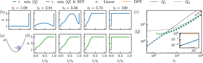
laboratory. RESULTS ACTIVE PARTICLE IN A TRAP OF VARIABLE STIFFNESS In this section we consider the problem of Section IIIA of ref. 51, a single active Ornstein-Uhlenbeck particle65,66,67 in

a one-dimensional harmonic trap of stiffness _α_(_t_). A schematic of this model is shown in Fig. 1a. The particle has position _r_ and self-propulsion velocity _v_. It experiences

overdamped Brownian motion with diffusion constant _D_ and mobility _μ_, such that $$\dot{r}(t)=v(t)-\mu \alpha \,r(t)+\sqrt{2D}\eta (t).$$ (1) Here _η_ is a Gaussian white noise term with

zero mean and unit variance. The self-propulsion velocity _v_ follows an Ornstein-Uhlenbeck process with persistence time _τ_ and amplitude _D_1, such that \(\left\langle v\right\rangle=0\)

and \(\left\langle v(t)v({t}^{{\prime} })\right\rangle={D}_{1}{\tau }^{-1}{e}^{-| t-{t}^{{\prime} }| /\tau }\). The parameter _D_1 is zero in the passive limit. The trajectory-averaged heat

associated with varying _α_(_t_) from _α_i to _α_f in time _t_f is19,51,66 $$\left\langle Q\right\rangle= \frac{1}{2}\left({\alpha }_{{{{\rm{i}}}}}{x}_{{{{\rm{i}}}}}-{\alpha

}_{{{{\rm{f}}}}}{x}_{{{{\rm{f}}}}}\right)+\frac{1}{2}\int_{0}^{{t}_{{{{\rm{f}}}}}}{{{\rm{d}}}}t\,\dot{\alpha }(t)x(t)\\ +\frac{{D}_{1}{t}_{{{{\rm{f}}}}}}{\tau \mu

}-\int_{0}^{{t}_{{{{\rm{f}}}}}}{{{\rm{d}}}}t\,\alpha (t)y(t).$$ (2) Here \(\left\langle \cdot \right\rangle\) denotes an average over dynamical trajectories, and we have defined \(x\equiv

\left\langle {r}^{2}\right\rangle\) and \(y\equiv \left\langle rv\right\rangle\). For time-dependent quantities _q_(_t_) we use the notation _q_i ≡ _q_(0) and _q_f ≡ _q_(_t_f) to denote

initial and final values. The first line of Eq. (2) is the passive heat (minus the change in energy plus the work done by changing the trap stiffness), and the second line is the active

contribution to the heat. The first term on the second line is constant for fixed _t_f (describing the heat dissipated to sustain the self-propelled motion), and plays no role in selecting

the protocol. For a given protocol _α_(_t_), the time evolution of _x_ and _y_ is given by the equations51 $$\frac{1}{2}\,\dot{x}(t)+\mu \alpha (t)x(t) =y(t)+D,\,\,{{{\rm{and}}}}\\ \tau

\dot{y}(t)+\gamma (t)y(t) ={D}_{1},$$ (3) where _γ_(_t_) ≡ 1 + _μ__τ__α_(_t_). The system starts in the steady state associated with the trap stiffness _α_i, and so its initial coordinates

are $${x}_{{{{\rm{i}}}}}=\frac{1}{{\alpha }_{{{{\rm{i}}}}}\mu }\left(\frac{{D}_{1}}{{\gamma }_{{{{\rm{i}}}}}}+D\right)\,\,{{{\rm{and}}}}\,\,\,{y}_{{{{\rm{i}}}}}=\frac{{D}_{1}}{{\gamma

}_{{{{\rm{i}}}}}}.$$ (4) Ref. 51 sought protocols that carry out the change of trap stiffness _α_i = 1 → _α_f = 5 with minimum mean heat, Eq. (2). The theoretical framework used in that work

assumes that protocols _α_(_t_) are smooth and are not rapidly varying (see Section S2 for a discussion of this point). Here we revisit this problem using neuroevolution. We find that

heat-minimizing protocols are not in general slowly varying or smooth, but can vary rapidly and can display jump discontinuities. The protocols we identify produce considerably less heat

than do the protocols identified in ref. 51 (see Fig. 1 and Fig. S2). To learn a protocol _α_(_t_) that minimizes heat, we encode a general time-dependent protocol using a deep neural

network. We choose the parameterization $${\alpha }_{{{{\boldsymbol{\theta }}}}}(t)={\alpha }_{{{{\rm{i}}}}}+({\alpha }_{{{{\rm{f}}}}}-{\alpha

}_{{{{\rm{i}}}}})(t/{t}_{{{{\rm{f}}}}})+{g}_{{{{\boldsymbol{\theta }}}}}(t/{t}_{{{{\rm{f}}}}}),$$ (5) where _g_ is the output of a neural network whose input is _t_/_t_f (restricting the

scale of inputs to a range [0, 1] typically allows training to proceed faster than when inputs can be numerically large). We constrain the neural network so that _α_i ≤ _α__Θ_(_t_) ≤ _α_f,

meaning that it cannot access values of _α_ outside the range studied in ref. 51. When we relax this constraint we find protocols that produce less heat, in general, than the protocols that

observe the constraint. We impose the constraint to allow us to make contact with ref. 51, and because experimental systems have constraints on the maximum values of their control

parameters. Initially the weights and output of the neural network are zero, and so we start by assuming a protocol that interpolates linearly with time between the initial and final values

of _α_. We train the neural network by genetic algorithm to minimize the order parameter \(\phi=\left\langle Q\right\rangle\), given by Eq. (2), which we calculate for a given protocol by

propagating (3) for time _t_f, using a forward Euler discretization with step Δ_t_ = 10−3. An example of the learning process is shown in Fig. S2a. In Fig. 1b we show, for the choice _D_1 = 

2, that heat-minimizing protocols learned by the neural network vary between a step-like jump at the final time, for small values of _t_f, and a step-like jump at the initial time, for large

values of _t_f (all protocols shown in this work are provided in the Supplementary Data 1 file). For intermediate values of _t_f we observe a range of protocol types. These protocols

include non-monotonic and rapidly-varying forms, and show jump discontinuities at initial and final times. In Sec. S3A, we discuss the effect of the model parameters on the range of _t_f for

which these non-trivial protocols result in a lower value of 〈_Q_〉 than the step protocols. The heat associated with the final-time step protocol is just that associated with the initial

steady state, and is $${Q}_{1}=\frac{{D}_{1}{t}_{{{{\rm{f}}}}}}{\mu \tau \, (1+{\alpha }_{{{{\rm{i}}}}}\mu \tau )}.$$ (6) The heat associated with the initial-time jump protocol can be

calculated from Eqs. (2) and (3), and is $${Q}_{2}= \frac{{\alpha }_{{{{\rm{f}}}}}}{2}\left({x}_{{{{\rm{i}}}}}-{x}_{2}({t}_{{{{\rm{f}}}}})\right)+\frac{{D}_{1}{t}_{{{{\rm{f}}}}}}{\mu \tau

(1+{\alpha }_{{{{\rm{f}}}}}\mu \tau )}\\ -\frac{{D}_{1}\tau {\alpha }_{{{{\rm{f}}}}}}{{\gamma }_{{{{\rm{f}}}}}}\left(\frac{1}{{\gamma }_{{{{\rm{i}}}}}}-\frac{1}{{\gamma

}_{{{{\rm{f}}}}}}\right)\left(1-{{{{\rm{e}}}}}^{-{\gamma }_{{{{\rm{f}}}}}{t}_{{{{\rm{f}}}}}/\tau }\right),$$ (7) where $${x}_{2}(t)\equiv \,

({x}_{{{{\rm{i}}}}}-{x}_{{{{\rm{f}}}}}){{{{\rm{e}}}}}^{-2\mu {\alpha }_{{{{\rm{f}}}}}t}+{x}_{{{{\rm{ss}}}}}\\ +2{D}_{1}\left(\frac{1}{{\gamma }_{{{{\rm{i}}}}}}-\frac{1}{{\gamma

}_{{{{\rm{f}}}}}}\right){\left(2\mu {\alpha }_{{{{\rm{f}}}}}-\frac{{\gamma }_{{{{\rm{f}}}}}}{\tau }\right)}^{-1}\\ \times \left({{{{\rm{e}}}}}^{-{\gamma }_{{{{\rm{f}}}}}t/\mu

}-{{{{\rm{e}}}}}^{-2\mu {\alpha }_{{{{\rm{f}}}}}t}\right).$$ (8) Note that _x_ss is given in Eq. (10). For large _t_f we have $${Q}_{2}\approx \frac{{D}_{1}{t}_{{{{\rm{f}}}}}}{\mu \tau

(1+{\alpha }_{{{{\rm{f}}}}}\mu \tau )},$$ (9) which is the heat associated with the final steady state. In Fig. 1c we show that the heat values associated with the trained neural-network

protocols interpolate, as a function of _t_f, between the values _Q_1 and _Q_2. Our conclusion is that this optimization problem is solved by protocols that are rapidly varying, have a

variety of functional forms, and display jump discontinuities. As shown in the inset of Fig. 1c and in Fig. S2, these protocols produce values of heat considerably smaller than those

associated with the protocols derived in ref. 51. (In the latter figure we also show that it is possible to construct smooth but rapidly-varying protocols that can produce values of heat

arbitrarily close to the discontinuous protocols identified by the learning procedure). The protocols just described are valid solutions to the heat-minimization problem defined in ref. 51.

However, some of them are not meaningful in experimental terms. For instance, for small values of _t_f, the heat-minimizing protocol is a step function at the final time. This protocol is a

solution to the stated problem, but effects no change of the system’s microscopic coordinates. All the heat associated with the subsequent transformation of the system is ignored, simply

because we have stopped the clock. We therefore argue that it is more meaningful to search for protocols that minimize heat subject to the requirement of a state-to-state transformation.

That is, we require that a specified change in the system’s state has occurred. We modify the problem studied in ref. 51 to search for protocols that minimize the mean heat (2) caused by a

change of trap stiffness _α_i = 1 → _α_f = 5, subject to the completion of a state-to-state transformation (SST) between the initial steady state (4) and that associated with the final-time

value of _α_f, $${x}_{{{{\rm{ss}}}}}=\frac{1}{{\alpha }_{{{{\rm{f}}}}}\mu }\left(\frac{{D}_{1}}{{\gamma

}_{{{{\rm{f}}}}}}+D\right)\,\,{{{\rm{and}}}}\,\,\,{y}_{{{{\rm{ss}}}}}=\frac{{D}_{1}}{{\gamma }_{{{{\rm{f}}}}}}.$$ (10) As before, we impose the experimentally-motivated constraint _α_i ≤

_α__Θ_(_t_) ≤ _α_f. To solve this dual-objective problem we choose the evolutionary order parameter $$\phi=\Delta+c\,\,{{{\rm{if}}}}\,\Delta \ge {\Delta

}_{0}\,\,{{{\rm{and}}}}\,\,\phi=\left\langle Q\right\rangle \,{{{\rm{otherwise}}}}.$$ (11) Here \({\Delta }^{2}\equiv

{({x}_{{{{\rm{f}}}}}-{x}_{{{{\rm{ss}}}}})}^{2}+{({y}_{{{{\rm{f}}}}}-{y}_{{{{\rm{ss}}}}})}^{2}\) measures the difference between the final-time system coordinates and their values (10) in the

final steady state; Δ0 = 10−3 is the tolerance with which we wish to achieve this steady state; and _c_ = 100 is an arbitrary constant whose only role is to make the first clause of (11)

always larger than the second (protocols and heat values depend weakly on the value of the threshold Δ, but not in a way that affects our general conclusions). Minimizing (11) will minimize

heat emission for a protocol _α_(_t_) that in time _t_f effects a state-to-state transformation within the precision Δ0. In Fig. 1d we show protocols that minimize heat while achieving SST

(see also Sec. S4). These protocols have a variety of forms, which involve rapidly-varying portions and jump discontinuities, and that tend, for large _t_f, to the initial-time jump form.

For times _t_f ≲ 1.3 the learning algorithm could not identify a protocol that could achieve SST. We discuss how this minimal time is affected by the model parameters in Sec. S3B. The heat

emission associated with these protocols is shown in panel (c). The time _t_f for which least heat is emitted is about _t_f = 1.74, for this choice of _D_1. (For heat optimization alone, the

minimum heat is \(\left\langle Q\right\rangle=0\), and is shown by Eq. (6) to occur at time _t_f = 0, a conclusion different to that drawn in Fig. 3 of ref. 51. This strange result follows

from the fact that the instruction to minimize heat comes with no requirement that the system change state.) For comparison, we show the heat emission associated with the linear protocol

_α_lin(_t_) = _α_i + (_α_f − _α_i)(_t_/_t_f) (square symbols). The linear protocol emits considerably more heat than learned protocols (note the log scale of the figure), and fails to

achieve SST for times _t_f ≲ 60. We conclude that the model of the confined active particle studied in ref. 51 is best controlled by protocols _α_(_t_) that are in general rapidly varying

and exhibit jump discontinuities – similar to protocols for overdamped passive systems – whether the goal is to minimize heat or to do so while also inducing SST. We note that while the

evolutionary training of the neural network is a numerical procedure, the protocols it identified allowed us to derive analytic results for the minimum heat produced for sufficiently small

and large trajectory lengths, Eq. (6) and Eq. (7) respectively. ACTIVE PARTICLE OF VARIABLE ACTIVITY IN A TRAP OF VARIABLE STIFFNESS STATE-TO-STATE TRANSFORMATION IN LEAST TIME In this

section we consider the problem of ref. 52, an active Brownian particle confined by a two-dimensional harmonic potential \(U({{{\boldsymbol{\rho }}}})=\frac{1}{2}k{{{{\boldsymbol{\rho

}}}}}^{2}\) with stiffness _k_. The particle is described by the position vector \({{{\boldsymbol{\rho }}}}=(\rho \cos \phi,\rho \sin \phi )\) and orientation _θ_, and moves in the direction

\(\hat{{{{\boldsymbol{e}}}}}(\theta )=(\cos \theta,\sin \theta )\) with constant speed _u_0. Its dynamics is described by the Langevin equation $$\frac{{{{\rm{d}}}}{{{\boldsymbol{\rho

}}}}}{{{{\rm{d}}}}\tau } \,={u}_{0}\hat{{{{\boldsymbol{e}}}}}(\theta )-\mu k{{{\boldsymbol{\rho }}}}+\sqrt{2{D}_{t}}{{{{\boldsymbol{\xi }}}}}_{r}(\tau )\\ \frac{{{{\rm{d}}}}\theta

}{{{{\rm{d}}}}\tau } \,=\sqrt{2{D}_{\theta }}{\xi }_{\theta }(\tau ),$$ (12) where _τ_ is the time; _μ_ is the mobility; _D__t_ and _D__θ_ are translational and rotational diffusion

coefficients, respectively; and _Ξ__r_(_τ_) and _ξ__θ_(_τ_) are Gaussian white noise terms with zero mean and unit variance. Upon introducing the dimensionless variables

\({{{\boldsymbol{r}}}}\equiv {{{\boldsymbol{\rho }}}}\sqrt{{D}_{\theta }/{D}_{t}}\) and _t_ ≡ _τ__D__θ_, Eq. (12) reads $$\frac{{{{\rm{d}}}}{{{\boldsymbol{r}}}}}{{{{\rm{d}}}}t} \,=\lambda

\hat{{{{\boldsymbol{e}}}}}(\theta )-\kappa {{{\boldsymbol{r}}}}+\sqrt{2}{{{{\boldsymbol{\xi }}}}}_{r}(t)\\ \frac{{{{\rm{d}}}}\theta }{{{{\rm{d}}}}t} \,=\sqrt{2}{\xi }_{\theta }(t),$$ (13)

where _κ_ ≡ _μ__k_/_D__θ_ and \(\lambda \equiv {u}_{0}/\sqrt{{D}_{\theta }{D}_{t}}\) are dimensionless versions of the spring constant and the self-propulsion speed (_λ_ is the Péclet

number). These dimensionless variables are the control parameters of the problem. The steady-state probability distribution function \({{{{\mathcal{P}}}}}_{{{{\rm{ss}}}}}(r,\chi )\) of the

system depends only on _r_ ≡ ∣_R_∣ and _χ_ ≡ _θ_ − _ϕ_, and is known exactly68. The steady state associated with the control-parameter choices _κ_ and _λ_ can be classified as passive or

active (Fig. 2a): in the passive phase, the radial probability distribution _P_(_r_) is peaked at the trap center, while in the active phase it is peaked at _r_ > 0. This model system is

motivated by experiments involving spherical Janus particles, whose self-propulsion speed can be tuned through light intensity9, confined in a trap constructed by acoustic waves69. For a

typical experimental setup the control parameters are bounded as 0 ≤ _λ_ ≤ 11 and 1 ≤ _κ_ ≤ 79,52,69. The problem described in ref. 52 is to find a time-dependent protocol (_λ_(_t_), 

_κ_(_t_)) that obeys the bounds of the previous paragraph and that minimizes the time _t_f required to transform the distribution \({{{\mathcal{P}}}}(r,\chi )\) from a passive steady state

at (_λ_i, _κ_i) = (2.5, 4) to an active one at (_λ_f, _κ_f) = (5, 4). Using an ansatz constrained so that the distribution \({{{\mathcal{P}}}}(r(t),\chi (t))\) has at all times the form of

the steady-state distribution \({{{{\mathcal{P}}}}}_{{{{\rm{ss}}}}}(r,\chi )\) with effective values for the control parameters, the authors of that paper found a protocol that completed the

state-to-state transformation in time _t_f ≈ 0.44. This was achieved by inserting this ansatz into the Fokker-Planck equation for the time evolution of the probability distribution. In

order for analytical calculations to be feasible, one also has to assume that the effective value of the stiffness is constant throughout time. Under these assumptions, the protocol for the

activity _λ_ is determined solely by the protocol for the stiffness _κ_, see Eq. (6) in ref. 52. The resulting protocol is shown in Fig. 2a, b. A neural-network ansatz for the protocol is

free of the restrictions required for the analytical calculations: it does not assume a functional form for the probability distribution at intermediate times, and the protocols for _λ_(_t_)

and _κ_(_t_) are independent. With a trained neural-network ansatz for the protocol (_λ_(_t_), _κ_(_t_)), we find that the state-to-state transformation can be achieved about three times as

rapidly as it is under the analytic protocol of ref. 52. For a simulation of fixed time _t_f we use a genetic algorithm to train the neural network to minimize the order parameter _ϕ_ = Δ,

the mean-squared error between the target distribution \({{{{\mathcal{P}}}}}_{{{{\rm{ss}}}}}^{\star }(r,\chi )\) associated with the control-parameter values (_λ_f, _κ_f) and the

distribution \({{{\mathcal{P}}}}(r({t}_{{{{\rm{f}}}}}),\chi ({t}_{{{{\rm{f}}}}}))\) obtained at the end of the simulation. The latter was calculated from 105 independent trajectories of (13)

under a given neural-network protocol. The protocol learned by the neural network for time _t_f = 0.16 is shown in Fig. 2a, b, together with the protocol of ref. 52. Both show sharp jumps

in trap stiffness, decreasing it abruptly to its smallest possible value (we discuss the effect of the control parameter ranges on the learned protocols in Sec. S3C). The neural-network

protocol achieves the transformation more quickly because it also enacts a sharp jump in activity, setting it to the maximum possible value (the constraints imposed in ref. 52 mean that if

one control parameter achieves its maximum value in an abrupt way, the other is not free to do so). Near the end of the learned protocol both parameters are abruptly changed to their final

values. In Fig. 2c, we show the temporal evolution of _P_(_r_) for the learned protocol. Starting from an initial distribution peaked at the origin, the peak of _P_(_r_) overshoots the peak

of the target distribution (they are not at that time of the same shape). The peak of _P_(_r_) is later brought back toward the target when stiffness and activity are set to their maximal

and minimal values, respectively. Subsequently, both are set to their final values. In Fig. 2d, we show the final-time distribution of _χ_ for the learned protocol, which matches the target

distribution. In Fig. 2e we show the value of Δ obtained by protocols trained at various fixed simulation times _t_f. For times _t_f ≳ 0.15, the learned protocol produces a small constant

value of Δ consistent with the value produced by the protocol of ref. 52 (horizontal line). For times _t_f ≲ 0.15 the value of Δ increases sharply with decreasing _t_f, indicating that the

state-to-state transformation cannot be achieved with the same precision. STATE-TO-STATE TRANSFORMATION WITH WORK EXTRACTION It is possible to extract work during the state-to-state

transformation. Setting _t_f = 0.44, the transformation time of the protocol of ref. 52, we used a genetic algorithm to train a neural network to minimize the objective

$$\phi=\Delta+c\,\,{{{\rm{if}}}}\,\Delta \ge {\Delta }_{0}\,\,{{{\rm{and}}}}\,\,\phi=\left\langle W\right\rangle \,{{{\rm{otherwise}}}}.$$ (14) Here Δ0 is the mean-squared error associated

with the protocol of ref. 52 (calculated using 105 trajectories), and _c_ = 100 is an arbitrary constant whose only role is to make the first clause of (14) always larger than the second.

The quantity \(\left\langle W\right\rangle\) is the mean work, in units of _μ_/_D__t_, given by $$\langle W\rangle=\int_{0}^{{t}_{{{{\rm{f}}}}}}{{{\rm{d}}}}t\,\dot{\kappa }\left\langle

\frac{\partial U}{\partial \kappa }\right\rangle=\frac{1}{2}\int_{0}^{{t}_{{{{\rm{f}}}}}}{{{\rm{d}}}}t\,\dot{\kappa }\left\langle {r}^{2}\right\rangle .$$ (15) Minimizing (14) will minimize

the mean work associated with a protocol (_λ_(_t_), _κ_(_t_)) that in time _t_f effects the state-to-state transformation to a precision Δ0. The protocol learned in this way is shown in Fig.

 3a, b, together with the protocol of ref. 52. Panels (c) show the effect of the learned protocol on the radial probability distribution. The neural-network protocol increases _κ_ to its

maximum value at the beginning of the protocol. Doing so costs work, but only small amounts because the system is initially in a passive phase and so 〈_r_2〉 is small. The protocol also

increases _λ_ to a large (but sub-maximal) value, which begins to drive the distribution into the active phase, so increasing 〈_r_2〉. Subsequently, _κ_ is decreased to its target value,

causing a decrease of energy and allowing net extraction of work. Figure 3d shows the work distributions _P_(_W_) associated with the learned protocol and that of ref. 52. The latter results

in a broad distribution of work values, and on average requires a large input of work to enact the transformation. By contrast, the work distribution obtained using the learned protocol is

sharply peaked at a negative value, and the mean work is negative. In Fig. 3e we show mean work as a function of time for the two protocols. The learned protocol requires an input of work at

early times in order to extract net work at later times. This solution was identified by a genetic algorithm using an order parameter (14) that depends only on quantities evaluated at the

final time point. As a result, the protocol is not biased toward any particular functional form. By contrast, greedy reinforcement-learning algorithms, which at all times attempt to reduce

the objective function, would (without special shaping of the reward function) be unlikely to find the solution shown here. WORK EXTRACTION FROM CONFINED, INTERACTING ACTIVE PARTICLES We now

consider the case of _N_ interacting active Brownian particles placed within the two-dimensional harmonic trap of the previous section. Particle _i_ evolves according to the Langevin

equation $$\frac{{{{\rm{d}}}}{{{{\boldsymbol{r}}}}}_{i}}{{{{\rm{d}}}}t} =\lambda {\hat{{{{\boldsymbol{e}}}}}}_{i}(\theta )-\kappa {{{{\boldsymbol{r}}}}}_{i}-{\partial

}_{{{{{\boldsymbol{r}}}}}_{i}}\sum\limits_{j\ne i}V({r}_{ij})+\sqrt{2}{{{{\boldsymbol{\xi }}}}}_{r}(t)\\ \frac{{{{\rm{d}}}}{\theta }_{i}}{{{{\rm{d}}}}t} =\sqrt{2}{\xi }_{\theta }(t),$$ (16)

whose terms are similar to those of (12) with the addition of the Weeks-Chandler-Andersen interaction $$V(x)=\left\{\begin{array}{ll}4\epsilon \left[{\left(\sigma

/x\right)}^{12}-{\left(\sigma /x\right)}^{6}\right]+\epsilon \quad &(x \, < \, {2}^{1/6}\sigma )\\ 0\hfill \quad &({{{\rm{otherwise}}}}),\end{array}\right.$$ (17) which takes as

its argument the inter-particle separation _r__i__j_ ≡ ∣_R__j_ − _R__i_∣. We set _σ_ and _ϵ_ to 1. We wish to learn protocols that minimize the mean work done upon reducing the trap

stiffness from _κ_i = 5 to _κ_f = 2, in time _t_f, observing the bounds on the control parameter values as in the previous section. Here work is $$\langle

W\rangle=\frac{N}{2}\int_{0}^{{t}_{{{{\rm{f}}}}}}{{{\rm{d}}}}t\,\dot{\kappa }{R}^{2},$$ (18) where \({R}^{2}\equiv {N}^{-1}\mathop{\sum }_{i=1}^{N}\left\langle {r}_{i}^{2}\right\rangle\).

The angle brackets indicate an average over dynamical trajectories. We start from a steady state at _λ_i = 0, but place no constraints (beyond those of the control-parameter bounds) on the

value of _λ_f. Such a transformation could be used as part of a cycle for an active engine18,19,20. No analytical solutions are known for this many-body system, but a protocol can be learned

in exactly the same way as for the single-particle problems considered previously, using a genetic algorithm to train a neural network to minimize \(\phi=\left\langle W\right\rangle\). The

latter was calculated from 103 independent trajectories. In Fig. 4a we show the result of this learning procedure for trajectory time _t_f = 1 and a number of particles between _N_ = 1 and

_N_ = 40. In Figs. S7 and S8 we provide additional details of learned protocols for the cases _N_ = 12 and _N_ = 40. In all cases work can be extracted, \(\left\langle W\right\rangle \, <

\, 0\). However, the extracted work per particle is a non-monotonic function of _N_, attaining a minimum value for _N_ = 12. For this particular problem, the many-body system becomes more

efficient than the one-body system for _N_  > 25. This finding suggests that particular cycles of many-body active engines may function more efficiently with certain particle numbers. The

learned protocols that produce the work values in Fig. 4a initially increase _λ_ to its maximum value. For small _N_ they initially increase _κ_ to its maximum value, while for large _N_

they initially increase _κ_ to close to it maximum value (see Figs. S7 and S8). This initial increase of _κ_ costs work (as with the protocols in the previous section), but the significant

increase in _R_2 as the activity is increased allows for net work extraction upon the subsequent reduction of _κ_. As _N_ is increased from 1, the amount of work that can be extracted per

particle initially goes down. This decrease results from the fact that particles repel each other, and so _R_2 in the passive initial state is significantly larger for _N_ > 1 than for

_N_ = 1; see Fig. 4b. Increasing _κ_ (at early times) therefore costs more work per particle than for the case _N_ = 1. Work can still be extracted from this system, but less efficiently

than for the single-body system. For _N_ sufficiently large, however, the situation changes: _R_2 for large _λ_ and _κ_ becomes much larger than it is for a single particle (Fig. 4b, c) (for

small _N_, the value of _R_2 for large _λ_ and _κ_ is not much larger than it is for _N_ = 1, because particles spread out to form a ring and can adopt a mean radial position similar to

that preferred by a single particle). This change allows for greater work extraction per particle when _κ_ is decreased later on in the protocol. For _N_ > 25, this effect exceeds that

described in the previous paragraph, and the many-body system provides more work per particle than a one-body system. To illustrate the origin of the non-monotonicity seen in Fig. 4, we

consider a simplified protocol that instantaneously sets _κ_ and _λ_ to their maximum values, waits until the system reaches a steady state, and then sets _κ_ = _κ_f. The work per particle

associated with this protocol is given by $$\frac{{\langle W\rangle }_{{{{\rm{est}}}}}}{N}=\frac{1}{2}({\kappa }_{\max }-{\kappa }_{{{{\rm{i}}}}}){R}_{{\lambda }_{{{{\rm{i}}}}},{\kappa

}_{{{{\rm{i}}}}}}^{2}-\frac{1}{2}({\kappa }_{{{{\rm{f}}}}}-{\kappa }_{\max }){R}_{{\lambda }_{\max },{\kappa }_{\max }}^{2},$$ (19) where \({R}_{\lambda,\kappa }^{2}\) denotes the

steady-state value of _R_2 measured at (_λ_, _κ_). In Fig. 4c we show that Eq. (19) is a non-monotonic function of _N_. It is not a quantitatively accurate model of the learned protocols,

but captures one important feature of their behavior. Extending the simulation time to _t_f = 10 allows for even greater work extraction. This improvement is achieved by a learned protocol

that substantially changes the system’s activity twice, from passive to active to passive again (see Fig. S6). DISCUSSION We have shown that the efficient control of active-matter systems

generally requires protocols containing discontinuities and rapidly-varying features. We discuss how these can be obtained efficiently using neural networks trained with evolutionary

methods. We found protocols that achieve particular tasks – enacting state-to-state transformations or changing control parameters with minimal energy input – that were more efficient than

those derived recently by constrained analytical methods. Beyond these prototypical one-body problems, we showed that neural-network methods can aid in the design of protocols that achieve

extraction of work from many-body active systems. The approach we use is general and can be applied with relatively little modification to a wide variety of active-matter systems. For

instance, the optimization of active engines is a quickly growing field of research, garnering interest from both a numerical and experimental perspective18,19,20,21,22,23,24,25,26,27, and

our results demonstrate that neural networks can lead to optimal protocols for their control, for both interacting and non-interacting active particles. The learning scheme used here can be

applied to experiment the way it is applied to simulations, suggesting a way of designing protocols for the efficient manipulation of active matter in the laboratory. DATA AVAILABILITY The

protocols shown in this work are provided in the Supplementary Data 1 file. CODE AVAILABILITY An example of code for optimizing neural-network protocols for control problems in statistical

physics can be found in ref. 70. REFERENCES * Ramaswamy, S. The mechanics and statistics of active matter. _Annu. Rev. Condens. Matter Phys._ 1, 323–45 (2010). Article  ADS  Google Scholar 

* Romanczuk, P., Bär, M., Ebeling, W., Lindner, B. & Schimansky-Geier, L. Active brownian particles. _Eur. Phys. J. Spec. Top._ 202, 1–162 (2012). Article  CAS  Google Scholar  *

Marchetti, M. C. et al. Hydrodynamics of soft active matter. _Rev. Mod. Phys._ 85, 1143 (2013). Article  ADS  CAS  Google Scholar  * Bechinger, C. et al. Active particles in complex and

crowded environments. _Rev. Mod. Phys._ 88, 045006 (2016). Article  ADS  MathSciNet  Google Scholar  * Cavagna, A. & Giardina, I. Bird flocks as condensed matter. _Annu. Rev. Condens.

Matter Phys._ 5, 183–207 (2014). Article  ADS  CAS  Google Scholar  * Elgeti, J., Winkler, R. G. & Gompper, G. Physics of microswimmers—single particle motion and collective behavior: a

review. _Rep. Prog. Phys._ 78, 056601 (2015). Article  ADS  MathSciNet  CAS  PubMed  Google Scholar  * Needleman, D. & Dogic, Z. Active matter at the interface between materials science

and cell biology. _Nat. Rev. Mater._ 2, 1–14 (2017). Article  Google Scholar  * Zöttl, A. & Stark, H. Emergent behavior in active colloids. _J. Phys.: Condens. Matter_ 28, 253001 (2016).

ADS  Google Scholar  * Buttinoni, I., Volpe, G., Kümmel, F., Volpe, G. & Bechinger, C. Active brownian motion tunable by light. _J. Phys.: Condens. Matter_ 24, 284129 (2012). PubMed 

Google Scholar  * Cates, M. E. & Tailleur, J. Motility-induced phase separation. _Annu. Rev. Condens. Matter Phys._ 6, 219 (2015). Article  ADS  CAS  Google Scholar  * O’Byrne, J.,

Solon, A., Tailleur, J. & Zhao, Y. An Introduction to Motility-induced Phase Separation, in _Out-of-equilibrium Soft Matter_. https://doi.org/10.1039/9781839169465-00107 (The Royal

Society of Chemistry, 2023). * Toner, J., Tu, Y. & Ramaswamy, S. Hydrodynamics and phases of flocks. _Ann. Phys._ 318, 170–244 (2005). Article  ADS  MathSciNet  CAS  Google Scholar  *

Chaté, H. Dry aligning dilute active matter. _Annu. Rev. Condens. Matter Phys._ 11, 189–212 (2020). Article  ADS  Google Scholar  * Be’er, A. & Ariel, G. A statistical physics view of

swarming bacteria. _Mov. Ecol._ 7, 1–17 (2019). Article  Google Scholar  * Liebchen, B. & Levis, D. Collective behavior of chiral active matter: Pattern formation and enhanced flocking.

_Phys. Rev. Lett._ 119, 058002 (2017). Article  ADS  PubMed  Google Scholar  * Liebchen, B. & Löwen, H. Synthetic chemotaxis and collective behavior in active matter. _Acc. Chem. Res._

51, 2982–2990 (2018). Article  CAS  PubMed  Google Scholar  * Palacci, J., Sacanna, S., Steinberg, A. P., Pine, D. J. & Chaikin, P. M. Living crystals of light-activated colloidal

surfers. _Science_ 339, 936–940 (2013). Article  ADS  CAS  PubMed  Google Scholar  * Ekeh, T., Cates, M. E. & Fodor, É. Thermodynamic cycles with active matter. _Phys. Rev. E_ 102,

010101 (2020). Article  ADS  MathSciNet  CAS  PubMed  Google Scholar  * Fodor, É. & Cates, M. E. Active engines: Thermodynamics moves forward. _Europhys. Lett._ 134, 10003 (2021).

Article  ADS  CAS  Google Scholar  * Kumari, A., Pal, P. S., Saha, A. & Lahiri, S. Stochastic heat engine using an active particle. _Phys. Rev. E_ 101, 032109 (2020). Article  ADS 

MathSciNet  CAS  PubMed  Google Scholar  * Cocconi, L., Knight, J. & Roberts, C. Optimal power extraction from active particles with hidden states. _Phys. Rev. Lett._ 131, 188301 (2023).

Article  ADS  MathSciNet  CAS  PubMed  Google Scholar  * Saha, T. K. et al. Information engine in a nonequilibrium bath. _Phys. Rev. Lett._ 131, 057101 (2023). Article  ADS  MathSciNet  CAS

  PubMed  Google Scholar  * Holubec, V., Steffenoni, S., Falasco, G. & Kroy, K. Active brownian heat engines. _Phys. Rev. Res._ 2, 043262 (2020). Article  CAS  Google Scholar  * Holubec,

V. & Marathe, R. Underdamped active brownian heat engine. _Phys. Rev. E_ 102, 060101 (2020). Article  ADS  MathSciNet  CAS  PubMed  Google Scholar  * Datta, A., Pietzonka, P. &

Barato, A. C. Second law for active heat engines. _Phys. Rev. X_ 12, 031034 (2022). CAS  Google Scholar  * Gronchi, G. & Puglisi, A. Optimization of an active heat engine. _Phys. Rev. E_

103, 052134 (2021). Article  ADS  MathSciNet  CAS  PubMed  Google Scholar  * Pietzonka, P., Fodor, É., Lohrmann, C., Cates, M. E. & Seifert, U. Autonomous engines driven by active

matter: Energetics and design principles. _Phys. Rev. X_ 9, 041032 (2019). CAS  Google Scholar  * Caprini, L., Cecconi, F., Maggi, C. & Marconi, U. M. B. Activity-controlled clogging and

unclogging of microchannels. _Phys. Rev. Res._ 2, 043359 (2020). Article  CAS  Google Scholar  * Ghosh, A., Xu, W., Gupta, N. & Gracias, D. H. Active matter therapeutics. _Nano Today_

31, 100836 (2020). Article  CAS  PubMed  PubMed Central  Google Scholar  * Luo, M., Feng, Y., Wang, T. & Guan, J. Micro-/nanorobots at work in active drug delivery. _Adv. Funct. Mater._

28, 1706100 (2018). Article  Google Scholar  * Norton, M. M., Grover, P., Hagan, M. F. & Fraden, S. Optimal control of active nematics. _Phys. Rev. Lett._ 125, 178005 (2020). Article 

ADS  MathSciNet  CAS  PubMed  Google Scholar  * Shankar, S., Scharrer, L. V. D., Bowick, M. J. & Marchetti, M. C. Design rules for controlling active topological defects. _Proc. Natl

Acad. Sci._ 121, e2400933121 (2024). Article  CAS  PubMed  PubMed Central  Google Scholar  * Floyd, C., Dinner, A. R. & Vaikuntanathan, S. Learning to control non-equilibrium dynamics

using local imperfect gradients. arXiv preprint arXiv:2404.03798 (2024). * Rubenstein, M., Ahler, C., Hoff, N., Cabrera, A. & Nagpal, R. Kilobot: A low cost robot with scalable

operations designed for collective behaviors. _Robot. Autonomous Syst._ 62, 966–975 (2014). Article  Google Scholar  * Yigit, B., Alapan, Y. & Sitti, M. Programmable collective behavior

in dynamically self-assembled mobile microrobotic swarms. _Adv. Sci._ 6, 1801837 (2019). Article  Google Scholar  * Balda, A. B., Argun, A., Callegari, A. & Volpe, G. Playing with active

matter. arXiv preprint arXiv:2209.04168 (2022) * Gupta, D., Klapp, S. H. L. & Sivak, D. A. Efficient control protocols for an active Ornstein-Uhlenbeck particle. _Phys. Rev. E_ 108,

024117 (2023). Article  ADS  MathSciNet  CAS  PubMed  Google Scholar  * Guéry-Odelin, D., Jarzynski, C., Plata, C. A., Prados, A. & Trizac, E. Driving rapidly while remaining in control:

Classical shortcuts from Hamiltonian to stochastic dynamics. _Rep. Prog. Phys._ 86, 035902 (2023). Article  ADS  MathSciNet  Google Scholar  * Chennakesavalu, S. & Rotskoff, G. M.

Probing the theoretical and computational limits of dissipative design. _J. Chem. Phys._ 155, 194114 (2021). * Shankar, S., Raju, V. & Mahadevan, L. Optimal transport and control of

active drops. _Proc. Natl Acad. Sci._ 119, e2121985119 (2022). Article  CAS  PubMed  PubMed Central  Google Scholar  * Monderkamp, P. A., Schwarzendahl, F. J., Klatt, M. A. & Löwen, H.

Active particles using reinforcement learning to navigate in complex motility landscapes. _Mach. Learn.: Sci. Technol._ 3, 045024 (2022). ADS  Google Scholar  * Nasiri, M. & Liebchen, B.

Reinforcement learning of optimal active particle navigation. _N. J. Phys._ 24, 073042 (2022). Article  MathSciNet  Google Scholar  * Nasiri, M., Löwen, H. & Liebchen, B. Optimal active

particle navigation meets machine learning. _Europhys. Lett._ 142, 17001 (2023). Article  ADS  CAS  Google Scholar  * Falk, M. J., Alizadehyazdi, V., Jaeger, H. & Murugan, A. Learning

to control active matter. _Phys. Rev. Res._ 3, 033291 (2021). Article  CAS  Google Scholar  * Schmiedl, T. & Seifert, U. Optimal finite-time processes in stochastic thermodynamics.

_Phys. Rev. Lett._ 98, 108301 (2007). Article  ADS  PubMed  Google Scholar  * Gomez-Marin, A., Schmiedl, T. & Seifert, U. Optimal protocols for minimal work processes in underdamped

stochastic thermodynamics. _J. Chem. Phys._ 129, 024114 (2008) * Blaber, S., Louwerse, M. D. & Sivak, D. A. Steps minimize dissipation in rapidly driven stochastic systems. _Phys. Rev.

E_ 104, L022101 (2021). Article  ADS  MathSciNet  CAS  PubMed  Google Scholar  * Zhong, A. & DeWeese, M. R. Limited-control optimal protocols arbitrarily far from equilibrium. _Phys.

Rev. E_ 106, 044135 (2022). Article  ADS  MathSciNet  CAS  PubMed  Google Scholar  * Whitelam, S. Demon in the Machine: Learning to Extract Work and Absorb Entropy from Fluctuating

Nanosystems. _Phys. Rev. X_ 13, 021005 (2023). MathSciNet  CAS  Google Scholar  * Engel, M. C., Smith, J. A. & Brenner, M. P. Optimal Control of Nonequilibrium Systems through Automatic

Differentiation. _Phys. Rev. X_ 13, 041032 (2023). CAS  Google Scholar  * Davis, L. K., Proesmans, K. & Fodor, É. Active matter under control: Insights from response theory. _Phys. Rev.

X_ 14, 011012 (2024). CAS  Google Scholar  * Baldovin, M., Guéry-Odelin, D. & Trizac, E. Control of Active Brownian Particles: An Exact Solution. _Phys. Rev. Lett._ 131, 118302 (2023).

Article  ADS  MathSciNet  CAS  PubMed  Google Scholar  * Whitelam, S. & Tamblyn, I. Learning to grow: Control of material self-assembly using evolutionary reinforcement learning. _Phys.

Rev. E_ 101, 052604 (2020). Article  ADS  CAS  PubMed  Google Scholar  * Whitelam, S. & Tamblyn, I. Neuroevolutionary learning of particles and protocols for self-assembly. _Phys. Rev.

Lett._ 127, 018003 (2021). Article  ADS  CAS  PubMed  Google Scholar  * Whitelam, S. How to train your demon to do fast information erasure without heat production. _Phys. Rev. E_ 108,

044138 (2023). Article  ADS  MathSciNet  CAS  PubMed  Google Scholar  * Holland, J. H. Genetic algorithms. _Sci. Am._ 267, 66–73 (1992). Article  ADS  Google Scholar  * Mitchell, M. _An

introduction to genetic algorithms_ (MIT press, 1998). * Such, F. P. et al. Deep neuroevolution: genetic algorithms are a competitive alternative for training deep neural networks for

reinforcement learning. arXiv preprint arXiv:1712.06567 (2017). * Whitelam, S., Selin, V., Park, S.-W. & Tamblyn, I. Correspondence between neuroevolution and gradient descent. _Nat.

Commun._ 12, 1–10 (2021). Article  Google Scholar  * Hornik, K., Stinchcombe, M. & White, H. Multilayer feedforward networks are universal approximators. _Neural Netw._ 2, 359–366

(1989). Article  Google Scholar  * Bahri, Y. et al. Statistical mechanics of deep learning. _Annu. Rev. Condens. Matter Phys._ 11, 501–528 (2020). Article  ADS  Google Scholar  * Rotskoff,

G. M. & Crooks, G. E. Optimal control in nonequilibrium systems: Dynamic riemannian geometry of the ising model. _Phys. Rev. E_ 92, 060102 (2015). Article  ADS  Google Scholar  *

Gingrich, T. R., Rotskoff, G. M., Crooks, G. E. & Geissler, P. L. Near-optimal protocols in complex nonequilibrium transformations. _Proc. Natl Acad. Sci._ 113, 10263–10268 (2016).

Article  ADS  CAS  PubMed  PubMed Central  Google Scholar  * Barros, N., Whitelam, S., Ciliberto, S. & Bellon, L. Learning efficient erasure protocols for an underdamped memory. arXiv

preprint arXiv:2409.15050 (2024). * Martin, D. et al. Statistical mechanics of active ornstein-uhlenbeck particles. _Phys. Rev. E_ 103, 032607 (2021). Article  ADS  MathSciNet  CAS  PubMed 

Google Scholar  * Fodor, É., Jack, R. L. & Cates, M. E. Irreversibility and biased ensembles in active matter: Insights from stochastic thermodynamics. _Annu. Rev. Condens. Matter Phys._

13, 215–238 (2022). Article  ADS  Google Scholar  * Bonilla, L. L. Active ornstein-uhlenbeck particles. _Phys. Rev. E_ 100, 022601 (2019). Article  ADS  MathSciNet  CAS  PubMed  Google

Scholar  * Malakar, K., Das, A., Kundu, A., Kumar, K. V. & Dhar, A. Steady state of an active Brownian particle in a two-dimensional harmonic trap. _Phys. Rev. E_ 101, 022610 (2020).

Article  ADS  MathSciNet  CAS  PubMed  Google Scholar  * Takatori, S. C., De Dier, R., Vermant, J. & Brady, J. F. Acoustic trapping of active matter. _Nat. Commun._ 7, 10694 (2016).

Article  ADS  CAS  PubMed  PubMed Central  Google Scholar  * Whitelam, S. Demon in the machine: learning to extract work and absorb entropy from fluctuating nanosystems,

https://doi.org/10.5281/zenodo.13777105 swhitelam/demon, (2022). Download references ACKNOWLEDGEMENTS Work at the Molecular Foundry was supported by the Office of Science, Office of Basic

Energy Sciences, of the U.S. Department of Energy under Contract No. DE-AC02-05CH11231. This research used resources of the National Energy Research Scientific Computing Center (NERSC), a

U.S. Department of Energy Office of Science User Facility located at Lawrence Berkeley National Laboratory, operated under Contract No. DE-AC02-05CH11231, and the Stevin Supercomputer

Infrastructure, provided by the VSC (Flemish Supercomputer Center), funded by Ghent University, FWO and the Flemish Government – department EWI. C.C. was supported through a Francqui

Fellowship of the Belgian American Educational Foundation, and by the US Department of Energy, Office of Science, Office of Basic Energy Sciences Data, Artificial Intelligence and Machine

Learning at DOE Scientific User Facilities program under Award Number 34532 (a digital twin for in silico spatiotemporally-resolved experiments). AUTHOR INFORMATION AUTHORS AND AFFILIATIONS

* Molecular Foundry, Lawrence Berkeley National Laboratory, 1 Cyclotron Road, Berkeley, CA, 94720, USA Corneel Casert & Stephen Whitelam * Department of Physics and Astronomy, Ghent

University, 9000, Ghent, Belgium Corneel Casert Authors * Corneel Casert View author publications You can also search for this author inPubMed Google Scholar * Stephen Whitelam View author

publications You can also search for this author inPubMed Google Scholar CONTRIBUTIONS C.C. performed the simulations. S.W. did the analytic work. C.C. and S.W. discussed the results and

wrote the paper. CORRESPONDING AUTHORS Correspondence to Corneel Casert or Stephen Whitelam. ETHICS DECLARATIONS COMPETING INTERESTS The authors declare no competing interests. PEER REVIEW

PEER REVIEW INFORMATION _Nature Communications_ thanks the anonymous reviewers for their contribution to the peer review of this work. A peer review file is available. ADDITIONAL INFORMATION

PUBLISHER’S NOTE Springer Nature remains neutral with regard to jurisdictional claims in published maps and institutional affiliations. SUPPLEMENTARY INFORMATION SUPPLEMENTARY INFORMATION

PEER REVIEW FILE DESCRIPTION OF ADDITIONAL SUPPLEMENTARY FILES SUPPLEMENTARY DATA 1 RIGHTS AND PERMISSIONS OPEN ACCESS This article is licensed under a Creative Commons

Attribution-NonCommercial-NoDerivatives 4.0 International License, which permits any non-commercial use, sharing, distribution and reproduction in any medium or format, as long as you give

appropriate credit to the original author(s) and the source, provide a link to the Creative Commons licence, and indicate if you modified the licensed material. You do not have permission

under this licence to share adapted material derived from this article or parts of it. The images or other third party material in this article are included in the article’s Creative Commons

licence, unless indicated otherwise in a credit line to the material. If material is not included in the article’s Creative Commons licence and your intended use is not permitted by

statutory regulation or exceeds the permitted use, you will need to obtain permission directly from the copyright holder. To view a copy of this licence, visit

http://creativecommons.org/licenses/by-nc-nd/4.0/. Reprints and permissions ABOUT THIS ARTICLE CITE THIS ARTICLE Casert, C., Whitelam, S. Learning protocols for the fast and efficient

control of active matter. _Nat Commun_ 15, 9128 (2024). https://doi.org/10.1038/s41467-024-52878-2 Download citation * Received: 07 May 2024 * Accepted: 19 September 2024 * Published: 23

October 2024 * DOI: https://doi.org/10.1038/s41467-024-52878-2 SHARE THIS ARTICLE Anyone you share the following link with will be able to read this content: Get shareable link Sorry, a

shareable link is not currently available for this article. Copy to clipboard Provided by the Springer Nature SharedIt content-sharing initiative