Reader TTS

ABSTRACT Quantifying hunting harvest is essential for numerous ecological topics, necessitating reliable estimates. We here propose novel analytical tools for this purpose. Using a

hierarchical Bayesian framework, we introduce models for hunting reports that accounts for different structures of the data. Focusing on Swedish harvest reports of red fox (_Vulpes vulpes_),

wild boar (_Sus scrofa_), European pine marten (_Martes martes_), and Eurasian beaver (_Castor fiber_), we evaluated predictive performance through training and validation sets as well as

Leave One Out Cross Validation. The analyses revealed that to provide reliable harvest estimates, analyses must account for both random variability among hunting teams and the effect of

hunting area per team on the harvest rate. Disregarding the former underestimated the uncertainty, especially at finer spatial resolutions (county and hunting management precincts).

Disregarding the latter imposed a bias that overestimated total harvest. We also found support for association between average harvest rate and variability, yet the direction of the

association varied among species. However, this feature proved less important for predictive purposes. Importantly, the hierarchical Bayesian framework improved previously used point

estimates by reducing sensitivity to low reporting and presenting inherent uncertainties. SIMILAR CONTENT BEING VIEWED BY OTHERS PRESENCE-ONLY DATA FOR WILD UNGULATES AND RED FOX IN SPAIN

BASED ON HUNTING YIELDS OVER A 10-YEAR PERIOD Article Open access 10 February 2025 THE CONTINGENT IMPACT OF WIND FARMS ON GAME MAMMAL DENSITY DEMONSTRATED IN A LARGE-SCALE ANALYSIS OF

HUNTING BAG DATA IN POLAND Article Open access 25 October 2024 THE ROLE OF INDIVIDUAL VARIABILITY ON THE PREDICTIVE PERFORMANCE OF MACHINE LEARNING APPLIED TO LARGE BIO-LOGGING DATASETS

Article Open access 17 November 2022 INTRODUCTION Game management rely on relevant and cost-efficient monitoring data of sufficient quality and spatial resolution. For many game species,

harvest statistics are the only observations available, making them essential to most management programs1. Reliable estimates are essential, and there is a demand for new statistical

approaches for this purpose. Harvest reporting systems vary among countries. For instance, reporting is compulsory in many European countries but voluntary in others. Examples of voluntary

reporting include the United Kingdom and Cyprus (all species) and Finland (most species)2. In Sweden, harvest reporting is voluntary for most game species but mandatory for species with

pre-determined harvest quotas, e.g. moose (_Alces alces_), red deer (_Cervus elaphus_) and large carnivores such as wolf (_Canis lupus_). Harvest of species without pre-determined harvest

quotas is regulated by adaptions of the length of the open season, which is decided by the Swedish government based on suggestions from the Swedish Environmental Protection Agency, whereas

harvest quotas are decided by the respective County Administrative board. However, the right to hunt and ownership of felled game belongs to the landowner (before it is felled‚ the game

belongs to no one). Almost all land suitable for hunting is occupied by hunting teams consisting of landowners and/or hunters leasing hunting rights. Hunting teams are typically

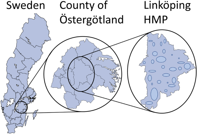
geographically stable over time, making it a suitable and stable unit for reporting. Teams annually report harvest and hunting area together with their geographic position to the level of

Hunting Management Precinct (HMP, Swedish: Jaktvårdskrets, N = 320 for the hunting year 2015/2016), geographic divisions based on the organisation of The Swedish Association for Hunting and

Wildlife Management (SAHWM). Hunting teams are encouraged via information meetings, social media, and magazines to report their harvest to the organisation. In this information, the

importance of reporting also if no game was felled (zero reports) is stressed. The NGO SAHWM has a public commission from the Swedish Government to provide annual harvest estimates for all

species with voluntary reporting. Data on harvest is made public online (www.viltdata.se) and is reported annually to the Swedish Government. The current estimation method extrapolates

linearly from reported harvest for each HMP, corresponding to the assumption that harvest rate is uniform within each HMP. While straightforward, the system has two major issues. First, it

provides only a point estimate without any measure of uncertainty. Second, it is potentially sensitive to low reporting rates, especially if intra-HMP variability among hunting teams is

prominent. At large spatial scales, harvest vary due to e.g. game species composition, game population density, and hunter abundance. At finer spatial scales, harvest variation may be caused

by e.g. microhabitat conditions or random variation in game preferences. Anecdotal observations have also indicated that harvest rate might be higher for small hunting areas compared to

larger ones. Bayesian statistics is well suited to analyse and transparently present uncertainties and is used increasingly in ecological research3. Because it is straightforward to carry

uncertainties forward to the prediction, it is a suitable system to estimate harvest for unreported hunting areas. An appealing feature of Bayesian analysis is the ability to tailor models

for the considered system and data. Specifically, Hierarchical Bayesian Modelling (HBM) allows analysts to address multiple levels of uncertainty4. Aiming at both system specific and general

insight, the purpose of this study is to introduce a Bayesian framework to improve hunting harvest estimation. We propose a set of Bayesian models and evaluate performance through training

and validation sets as well as Pareto Smoothed Importance Sampling Leave One Out Cross Validation (PSIS-LOO-CV)5. MATERIALS AND METHODS FOCAL SPECIES Currently, there are 49 species for

which SAHWM estimates annual harvest across Sweden. We focused on four species that exemplifies game harvested at high (H) or low (L) numbers and uniformly (U) or variably (V) across Sweden:

red fox (_Vulpes vulpes_, HU), wild boar (_Sus scrofa_, HV), European pine marten (_Martes martes_, LU), and Eurasian beaver (_Castor fiber_, LV). Red fox is one of the most abundant small

predators in the world6 and is common throughout Sweden, ranging from city parks to the high mountains. Red fox is harvested all over Sweden and is hunted for its pelt and to reduce

predation on other game species. The present Swedish wild boar population was established in the 1980s from escapes from enclosures and, likely, deliberate releases. Densities have increased

rapidly in recent years, causing great damage to agriculture. Wild boar is abundant in most of southern and central Sweden but absent from the northern parts of the country. Marten is

abundant throughout Sweden. It is an omnivore and the diet consist mainly of smaller animals, but also insects and berries. Marten is hunted for its pelt, often by specialized trappers.

Beaver was once eradicated in Sweden due to its valuable pelt but was reintroduced in the 1920s. It is tied to freshwater and eats bark and branches from hardwood trees. Beaver is present in

most of Sweden, except for the southernmost parts. It is hunted for its pelt, often by specialised trappers. DATA For each hunting year (July 1–June 30), hunting teams voluntarily report

their total harvest to SAHWM, most commonly through the SAHWM-owned database Viltdata (www.viltdata.se), with the opportunity to report their harvest continuously during the hunting year.

All reports are checked by local personnel of SAHWM, who, in doubtful cases, contacts the reporting person for clarifications. Examples of inconsistencies that are scrutinized are unusual

harvest numbers, no harvest (zero report) in areas where the species in question is common or reported harvest of a species outside its normal distribution area. The reported information

includes hunting area, number of individuals harvested for each species, and the HMP in which the hunting ground is located. Thus, HMP is the finest spatial resolution that can be considered

from the data. Levels of interest are illustrated in Fig. 1. All individual reports are confidential, and data is only presented at the HMP and higher levels. Here, we focused on hunting

data from 2015/2016, which included 5803 reports. The total reported area of 8,683,074 ha covered 26.5% of the total huntable area, meaning that harvest must be estimated for 73.5% of the

huntable area. As wild boar and beaver is not present in all of the country (wild boar not in the north and beaver not in the very south), we excluded counties where all reports indicated

zero harvest for the respective species. We also excluded HMPs for which SAHWM do not estimate harvest (north-western HMPs above the tree line and small, urban HMPs in Stockholm and

Uppsala). As such, the included HMPs varied among the species. CURRENT ESTIMATION METHOD The currently implemented model, henceforth denoted point estimate (P.E.), for hunting harvest in

Sweden extrapolates linearly from reports. Denoting with \(K_{r,k,l}\) and \(A_{r,k,l}\) harvest and hunting team area, respectively, for report _r_ in HMP _k_ in county _l_, the harvest per

area, \(\nu_{k,l}\) (animals ha−1), is calculated as $$\nu_{k,l} = \left\{ {\begin{array}{*{20}l} {\sum\limits_{{r \in {\mathbf{R}}_{k,l} }} {K_{r,k,l} } /\sum\limits_{{r \in

{\mathbf{R}}_{k,l} }} {A_{r,k,l} } \, } \hfill & {{\text{if }}\,{\text{there}}\,{\text{ is}}\,{\text{ at }}\,{\text{least }}\,{\text{one }}\,{\text{report}}\,{\text{ for}}\,{\text{

HMP}}\, \, k,l \, } \hfill \\ {\sum\limits_{{r \in {\mathbf{R}}_{l} }} {K_{r,k,l} } /\sum\limits_{{r \in {\mathbf{R}}_{l} }} {A_{r,k,l} } \, } \hfill & {{\text{if

}}\,{\text{there}}\,{\text{ is }}\,{\text{no}}\,{\text{ report }}\,{\text{for}}\,{\text{ HMP }}\,k,l} \hfill \\ \end{array} } \right.,$$ (1) where \({\mathbf{R}}_{k,l}\) is the set of

reports for HMP _k_ in county _l_, and \({\mathbf{R}}_{l}\) is the set of reports for county _l._ Denoting the total huntable area for HMP _k_ in county _l_ as \(T_{k,l}\) and defining the

corresponding unreported area as $$U_{k,l} = T_{k,l} - \sum\limits_{{r \in {\mathbf{R}}_{k,l} }} {A_{k,l} } ,$$ (2) the total estimated HMP harvest is estimated as $$E_{k,l} =

\sum\limits_{{r \in {\mathbf{R}}_{k,l} }} {K_{r,k,l} } + \nu_{k,l} U_{k,l} ,$$ (3) i.e. the sum of reported harvest for plus the estimated harvest for the unreported area. The nationwide

harvest is given by $$\ddot{E} = \sum\limits_{{l \in {\mathbf{l}}}} {\sum\limits_{{k \in {\mathbf{k}}_{l} }} {E_{k,l} } } .$$ (4) PROPOSED METHOD We propose Bayesian equivalents to the

current model. The analysis consists of three steps: analysis of reported hunting areas, analysis of reported harvest, and posterior prediction of unreported harvest volumes. ANALYSIS OF

REPORTED HUNTING AREAS We modelled the set of reported hunting areas A such that the area of report _r_ in HMP _k_ in county _l_ was modelled as $$A_{r,k,l} \sim \text{Log-Normal}\left(

{\log \left( {m_{k,l} } \right),s_{l} } \right),$$ (5) where \(\log \left( {m_{k,l} } \right)\) and \(s_{l}\) are the mean and standard deviation, respectively, of hunting areas on the

log-scale. We modelled \(m_{k,l}\) as $$m_{k,l} = \exp \left( {W + L_{l} + C_{k,l} } \right),$$ (6) where \(W\), \(L_{l}\), and \(C_{k,l}\) are the nationwide, county, and HMP level effects,

respectively. We further modelled. $$C_{k,l} \sim \text{Normal}\left( {0,t} \right),$$ (7) where _t_ is the standard deviation of HMP level effects and modelled as $$t \sim

\text{Log-Normal}\left( {\Omega_{t} ,S_{t} } \right).$$ (8) Similarly, county effects were modelled as $$L_{l} \sim \text{Normal}\left( {0,T} \right),$$ (9) where _T_ is the standard

deviation of county level effects and modelled with prior $$T \sim \text{Log-Normal}\left( {\Omega_{T} ,S_{T} } \right).$$ (10) We expressed the prior for the nationwide effect as $$W \sim

\text{Normal}\left( {\Omega_{W} ,S_{W} } \right).$$ (11) Because the model is expressed on the log-scale, \(s_{l}\) in Eq. (5) is a scale free measure of variability in hunting area within

each HMP. Exploratory analysis of the data suggested within HMP variability in hunting area per team—whether measured by variance or coefficient of variation—differed among counties. To

account for this pattern, we modelled \(s_{l}\) as $$s_{l} = \exp \left( {u + v_{l} } \right),$$ (12) where _u_ and \(v_{l}\) are interpreted as the nationwide and county level effects,

respectively, on the log-transform of this variability. County level effects on variability were modelled as $$v_{l} \sim \text{Normal}\left( {0,z} \right),$$ (13) where $$z \sim

\text{Log-Normal}\left( {\Omega_{z} ,S_{z} } \right).$$ (14) The prior for _u_ was modelled as $$u \sim \text{Normal}\left( {\Omega_{u} ,S_{u} } \right).$$ (15) BAYESIAN BASELINE MODEL FOR

REPORTED HARVEST As a first step towards a Bayesian model for harvest data, we assumed hunting within each HMP occurs uniformly with HMP specific rate (animals ha−1 yr−1), \(\mu_{k,l}\),

yielding the likelihood for the set of reports \({\mathbf{R}}_{k,l}\) $$P\left( {{\mathbf{R}}_{k,l} |\mu_{k,l} } \right) = \prod\limits_{{r \in {\mathbf{R}}_{k,l} }} {{\text{Poiss}} \left(

{K_{r,k,l} |\mu_{k,l} A_{r,k,l} } \right)} = {\text{Poiss}} \left( {\sum\limits_{{r \in {\mathbf{R}}_{k,l} }} {K_{r,k,l} } |\mu_{k,l} \sum\limits_{{r \in {\mathbf{R}}_{k,l} }} {A_{r,k,l} } }

\right).$$ (16) Solving $$\frac{{d\log \left( {P\left( {{\mathbf{R}}_{k,l} |\mu_{k,l} } \right)} \right)}}{{d\mu_{k,l} }} = \frac{1}{{\mu_{k,l} }}\sum\limits_{{r \in {\mathbf{R}}_{k,l} }}

{K_{r,k,l} } - \sum\limits_{{i \in {\mathbf{R}}_{k,l} }} {A_{r,k,l} } = 0,$$ (17) the maximum likelihood (ML) estimate for HMPs with at least one report is $$\hat{\mu }_{k,l} =

\sum\limits_{{r \in {\mathbf{R}}_{k,l} }} {K_{r,k,l} } /\sum\limits_{{r \in {\mathbf{R}}_{k,l} }} {A_{r,k,l} }$$ (18) Thus, the Poisson model is an obvious likelihood equivalent to Eq. (1).

Using a conjugate gamma prior, a posterior distribution for a Bayesian equivalent can be obtained as $$\begin{aligned} P\left( {\mu_{k,l} |{\mathbf{R}}_{k,l} } \right) & \propto

{\text{Poiss}} \left( {\sum\limits_{{r \in {\mathbf{R}}_{k,l} }} {K_{r,k,l} } |\mu_{k,l} \sum\limits_{{r \in {\mathbf{R}}_{k,l} }} {A_{r,k,l} } } \right){\text{Gamma}} \left( {\mu_{k,l}

|a,b} \right) \\ & \propto {\text{Gamma}} \left( {\mu_{k,l} |a + \sum\limits_{{r \in {\mathbf{R}}_{k,l} }} {K_{r,k,l} } ,b + \sum\limits_{{r \in {\mathbf{R}}_{k,l} }} {A_{r,k,l} } }

\right), \\ \end{aligned}$$ (19) where _a_ and _b_ are shape and rate parameters, respectively. However, the common approach to elicit vague priors as \(a = b =\) “something small” fails for

the focal system. Often, \(\sum\nolimits_{{r \in {\mathbf{R}}_{k,l} }} {K_{r,k,l} = 0}\), making the posterior of Eq. (19) sensitive to \(a\). Also, occasional HMP have no reports

(\(\sum\nolimits_{{r \in {\mathbf{R}}_{k,l} }} {A_{r,k,l} = 0}\)), making the posterior sensitive to \(b\). Thus, when reporting and/or harvest is low, it would be useful to borrow strength

from the harvest pattern in surrounding HMPs. We defined $$\log \left( {\mu_{k,l} } \right) = \chi_{k,l} + \lambda_{l} + \omega ,$$ (20) where \(\chi_{k,l}\), \(\lambda_{l}\) and \(\omega\)

are HMP, county and nationwide effects, respectively. This promotes a straightforward hierarchical structure for HMP and county effects as $$\begin{aligned} \chi_{k,l} & \sim

{\text{Normal}} \left( {0,\sigma } \right) \\ \lambda_{l} & \sim {\text{Normal}} \left( {0,\tau } \right), \\ \end{aligned}$$ (21) where \(\sigma\) and \(\tau\) are standard deviations

of HMP and county effects, respectively, and assigned priors $$\begin{aligned} \sigma & \sim \text{Log-Normal}\left( {\Omega_{\sigma } ,S_{\sigma } } \right) \\ \tau & \sim

\text{Log-Normal}\left( {\Omega_{\tau } ,S_{\tau } } \right). \\ \end{aligned}$$ (22) We refer to this Bayesian baseline model for harvest data as \({\rm M}_{0}\). WITHIN HMP VARIATION The

assumption of \({\rm M}_{0}\) that all hunting teams within an HMP harvests with equal rate \(\mu_{k,l}\) may be invalid. While underlying reasons for intra-HMP variability are for most part

intractable from the available data, non-homogeneous harvesting should be accounted for if it improves prediction. Thus, we specified an alternative likelihood $$\begin{aligned} &

P\left( {{\mathbf{R}}_{k,l} |\mu_{k,l} ,\alpha_{k,l} } \right) \\ & \quad = \prod\limits_{{r \in {\mathbf{R}}_{k,l} }} {\left[ {\frac{{\left( {{{\alpha_{k,l} } \mathord{\left/ {\vphantom

{{\alpha_{k,l} } {\left( {\mu_{k,l} A_{r,k,l} } \right)}}} \right. \kern-\nulldelimiterspace} {\left( {\mu_{k,l} A_{r,k,l} } \right)}}} \right)^{{\alpha_{k,l} }} }}{{\Gamma \left(

{K_{r,k,l} + 1} \right)\Gamma \left( {K_{r,k,l} + \alpha_{k,l} } \right)}}\frac{{\Gamma \left( {K_{r,k,l} + \alpha_{k,l} } \right)}}{{\left( {{{\alpha_{k,l} } \mathord{\left/ {\vphantom

{{\alpha_{k,l} } {\left( {\mu_{k,l} A_{r,k,l} } \right)}}} \right. \kern-\nulldelimiterspace} {\left( {\mu_{k,l} A_{r,k,l} } \right)}} + 1} \right)^{{K_{r,k,l} + \alpha_{k,l} }} }}}

\right],} \\ \end{aligned}$$ (23) which is the Gamma–Poisson mixture distribution parameterized from its mean \(\mu_{k,l} A_{r,k,l}\) and shape parameter \(\alpha_{k,l}\). This corresponds

to the assumption that hunting follows a Poisson process with a team specific rate, which is assumed to be gamma distributed. We keep the notation \(\mu_{k,l}\) as in Eq. (16) because the

Poisson distribution is the limiting case of the Gamma–Poisson mixture as \(\alpha_{k,l} \to \infty\), and for finite \(\alpha_{k,l}\), \(\mu_{k,l}\) is the average harvest rate for teams in

circuit _k_ in county _l_. The Gamma–Poisson mixture can be reparametrized as the Negative Binomial (NB), yet we use the Gamma–Poisson notation to avoid confusion with the standard

parameterization of the NB. We considered models for \(\alpha_{k,l}\) that either includes or excludes association between average harvest rate \(\mu_{k,l}\) and intra-HMP variation as

$$\log \left( {\alpha_{k,l} } \right) = \left\{ {\begin{array}{*{20}l} {\upsilon + \gamma \left( {\chi_{k,l} + \lambda_{l} } \right)} \hfill & {{\text{if}}\,{\text{

including}}\,{\text{rate--variability }}\,{\text{association}}} \hfill \\ \upsilon \hfill & {{\text{if }}\,{\text{excluding }}\,{\text{rate--variability }}\,{\text{association}}} \hfill

\\ \end{array} } \right.,$$ (24) where \(\gamma > 0\) indicates a positive effect of increased harvest rate (relative to nationwide average \(\omega\)) on the shape parameter

\(\alpha_{k,l}\). Large values of \(\alpha_{k,l}\) indicate less variability. We implemented priors $$\gamma \sim \text{Normal}\left( {\Omega_{\gamma } ,S_{\gamma } } \right)$$ (25)

$$\upsilon \sim \text{Normal}\left( {\Omega_{\upsilon } ,S_{\upsilon } } \right)$$ (26) and used the same hierarchical structure specified for \(\mu_{k,l}\) in \({\text{M}}_{0}\). EFFECT OF

HUNTING AREA ON HARVEST RATE We incorporated an additional parameter \(\phi\), modelling the potential effect of a team’s hunting area on its harvest rate per area, extending Eqs. (16) and

(23) to $$P\left( {{\mathbf{R}}_{k,l} |\mu_{k,l} ,\phi_{r,k,l} } \right) = \prod\limits_{{r \in {\mathbf{R}}_{k,l}}} {{\text{Poiss}} \left( {K_{r} |\mu_{k,l} A_{r} \delta_{r,k,l} }

\right)}$$ (27) and $$\begin{aligned} & P\left( {{\mathbf{R}}_{k,l} |\mu_{k,l} ,\alpha_{k,l} ,\phi_{r,k,l} } \right) \\ & \quad = \prod\limits_{{r \in {\mathbf{R}}_{k,l} }} {\left[

{\frac{{\left( {{{\alpha_{k,l} } \mathord{\left/ {\vphantom {{\alpha_{k,l} } {\left( {\delta_{r,k,l} \mu_{k,l} A_{r,k,l} } \right)}}} \right. \kern-\nulldelimiterspace} {\left(

{\delta_{r,k,l} \mu_{k,l} A_{r,k,l} } \right)}}} \right)^{{\alpha_{k,l} }} }}{{\Gamma \left( {K_{r,k,l} + 1} \right)\Gamma \left( {K_{r,k,l} + \alpha_{k,l} } \right)}}\frac{{\Gamma \left(

{K_{r,k,l} + \alpha_{k,l} } \right)}}{{\left( {{{\alpha_{k,l} } \mathord{\left/ {\vphantom {{\alpha_{k,l} } {\left( {\delta_{r,k,l} \mu_{k,l} A_{r,k,l} } \right)}}} \right.

\kern-\nulldelimiterspace} {\left( {\delta_{r,k,l} \mu_{k,l} A_{r,k,l} } \right)}} + 1} \right)^{{K_{r,k,l} + \alpha_{k,l} }} }}} \right]} , \\ \end{aligned}$$ (28) respectively, where

$$\delta_{r,k,l} = \exp \left( {\phi \log \left( {{{A_{r,k,l} } \mathord{\left/ {\vphantom {{A_{r,k,l} } {\overline{m}_{k,l} }}} \right. \kern-\nulldelimiterspace} {\overline{m}_{k,l} }}}

\right)} \right).$$ (29) Using \({{A_{r,k,l} } \mathord{\left/ {\vphantom {{A_{r,k,l} } {\overline{m}_{k,l} }}} \right. \kern-\nulldelimiterspace} {\overline{m}_{k,l} }},\) where

\(\overline{m}_{k,l}\) is the typical hunting team area in the focal HMP, facilitates the interpretation of \(\phi\) as the effect of relative hunting area and avoids confusing \(\phi\) with

large-scale differences in average hunting area among HMPs. To avoid refitting of the hunting area model for each species within each model of harvesting, we defined \(\overline{m}_{k,l}\)

as the median of the posterior of \(m_{k,l}\) defined in Eq. (6) For \(\phi = 0\), there is no effect of hunting area. For \(\phi < 0\), per area harvest rate decreases with hunting area.

We specified the prior $$\phi \sim \text{Normal}\left( {\Omega_{\phi } ,S_{\phi } } \right).$$ (30) MODEL NOTATION We denote with subscripts \(\alpha\), \(\gamma\), and/or \(\phi\) models

that include intra-HMP variability, association between harvest rate and intra-HMP variability, and/or effect of hunting area on harvest rate. Including \(\gamma\) is only relevant for

models including \(\alpha\). Thus, there are six considered Bayesian models: \({\rm M}_{\alpha \gamma \phi }\), \({\rm M}_{\alpha \phi }\), \({\rm M}_{\phi }\), \({\text{\rm M}}_{\alpha

\gamma }\),\({\rm M}_{\alpha }\), and \({\rm M}_{0}\). PRIOR ELICITATION Our approach was to specify ranges of parameter values that we deemed plausible across species. Defining this range

as the 95% central interval of the prior distribution, we allowed for posterior estimates outside of the range, should the likelihood strongly contradict our beliefs. The choice of Normal

and Log-Normal functional forms as priors were implemented because these distribution are suitable to incorporate (if however vague) prior beliefs, and we used the rule-of-thumb that ~ 95%

of the density lies within two standard deviations of the mean (accounting for the log-transform when using the Log-Normal). Table 1 lists prior parameters and the ranges from which they

were derived below. The highest-level parameters for the hunting area model are _W_, _T_, _t_, _u_, and _z_. The nationwide effect on average hunting area, _W_, is expressed for log-area,

and we specified the plausible range as [2.3, 9.2], corresponding to the vague prior belief that the typical hunting area per team is (with 95% certainty) between 10 and 10,000 ha. A

plausible range for the standard deviation of county effects on hunting area, _T_, can be derived from expectations about relative difference among counties. We knew there are geographic

differences and derived a lower range from the assumption that hunting areas in a county two standard deviations above or below the geometric average differ from the average by at least a

factor of 1.5. Conversely, we derived the upper range from the assumption that hunting areas in a county that is two standard deviations from the geometric average unlikely differs by more

than a factor of 100 from the average. The corresponding range on the log-scale used to parameterize the Log-Normal distribution is [0.20, 2.3]. We derived the prior of the standard

deviation of county effects, _t_, from similar expectations, yet with the lower and upper range at a factor of 1.1 and 20, respectively. The corresponding range on the log-scale is [− 1.3,

2.3]. Parameter _u_ models the nationwide effect on \(s_{l}\), the standard deviation of intra-HMP variability in hunting area per team. Expressing prior beliefs about this distribution is

more intuitive when considering its coefficient of variation, \(c = \sqrt {e^{{s_{l}^{2} }} - 1}\). We specified high and low variation as \(c = 10\) (standard deviation of hunting areas

within a HMP is ten times the average) and \(c = 0.1\) (standard deviation of hunting areas within an HMP is 10% of the average). This correspond to a range for _u_ as [− 2.3, 0.77].

Parameter _z_ models variability among counties in terms of intra-HMP variability. We expressed a plausible range based on relative difference between 0.1 (little variation among counties)

and 10 (high variation between counties), which corresponds to a range for _z_ between [0.095, 2.3]. The harvest rate models include up to six highest-level parameters: \(\omega\), \(\tau\),

\(\sigma\), \(\upsilon\), \(\gamma\), and \(\phi\). We derived the lower limit of the plausible range for \(\omega\) from the expectation that the geometric mean harvest rate corresponds to

at least one individual across Sweden’s approximately 32,800,000 ha of huntable land. We specified the upper limit from the expectation that the geometric mean rate is unlikely higher than

one animal per ha. The corresponding range for \(\omega\), which is expressed on the log-scale, is [− 17, 0]. Similar to _T_ and _t_, we derived plausible ranges for \(\tau\) and \(\sigma\)

from how effect sizes translates into relative difference among counties and HMPs, respectively. For variability of county effects \(\tau\), we assumed a plausible effect size at two

standard deviations from the geometric average between a factor of 1.5 and 100, corresponding to a prior range for \(\tau\) of [0.20, 2.3]. For \(\sigma\), modelling variability of HMPs

within a county, we specified plausible relative differences as between a factor of 1.1 and 20, which corresponds to a prior range of [− 1.3, 2.3]. For \(\upsilon\), the intercept of \(\log

\left( {\alpha_{k,l} } \right)\), we utilized the relationship between the Gamma–Poisson mixture’s shape parameter and the coefficient of variation of harvest rates described by the

associated Gamma distribution, \(c = {1 \mathord{\left/ {\vphantom {1 {\sqrt \alpha }}} \right. \kern-\nulldelimiterspace} {\sqrt \alpha }}\). Under high intra-HMP variability, we assumed

_c_ may be as high as 20. If variability is low, a plausible _c_ could be as low as 1/20. These upper and lower limits for _c_ translate to a range of the shape parameter within 0.025 and

400, respectively, which when log-transformed to the scale of \(\upsilon\) is [− 6.0, 6.0]. We further assumed \(\gamma\) should (with 95% certainty) be limited to an increase or decrease of

coefficient of variation with a factor of two with every doubling of the average harvest rate. This corresponds to a prior range for \(\gamma\) as [−2.0, 2.0]. If \(\phi = - 1\), there is

no change in the harvest rate per team with hunting area. If \(\phi = 1\), the harvest rate per team grows quadratically with hunting area. Thus, we let these extremes define the prior range

for \(\phi\). PREDICTION We performed posterior predictive sampling of harvest for the unreported area by repeatedly sampling team areas and team specific harvest rates according to each

candidate model for harvesting. The number of non-reporting hunting teams is unknown, but our framework permits us to sample recursively until we overshoot \(U_{k,l}\). To ensure a

consistent total area, we truncated the overshooting sample. Team level harvests are assumed to follow a Poisson process for all models, and we sampled $$K_{k,l}^{(q,h)} \sim {\text{Poiss}}

\left( {\theta_{k,l}^{(q,h)} } \right),$$ (31) where \(\theta_{k,l}^{(q,h)}\) is the harvest rate for sampled team _h_ for posterior sample _q_ and is assigned as $$\begin{aligned}

\theta_{k,l}^{(q,h)} & = A_{h} \mu_{k,l}^{(q)} \, \,{\text{for }}\,{\rm M}_{0} \\ \theta_{k,l}^{(q,h)} & \sim \text{Gamma}\left( {\alpha_{k,l}^{(q)} ,{{\mu_{k,l}^{(q)} A_{h} }

\mathord{\left/ {\vphantom {{\mu_{k,l}^{(q)} A_{h} } {\alpha_{k,l}^{(q)} }}} \right. \kern-\nulldelimiterspace} {\alpha_{k,l}^{(q)} }}} \right) \, \,{\text{for}}\, \, {\rm M}_{\alpha \gamma

} \, \,{\text{and }}\,{\rm M}_{\alpha } \\ \theta_{k,l}^{(q,h)} & = \mu_{k,l}^{(q)} A_{h} e^{{\log \left( {\overline{A}_{r} } \right)\phi^{(q)} }} \, \,{\text{for }}\,{\rm M}_{\phi } \\

\theta_{k,l}^{(q,h)} & \sim \text{Gamma}\left( {\alpha_{k,l}^{(q)} ,{{\mu_{k,l}^{(q)} A_{h} e^{{\log \left( {\overline{A}_{h} } \right)\phi^{(q)} }} } \mathord{\left/ {\vphantom

{{\mu_{k,l}^{(q)} A_{h} e^{{\log \left( {\overline{A}_{h} } \right)\phi^{(q)} }} } {\alpha_{k,l}^{(q)} }}} \right. \kern-\nulldelimiterspace} {\alpha_{k,l}^{(q)} }}} \right){\text{ for

}}\,{\rm M}_{\alpha \gamma \phi } \, \,{\text{and}}\, \, {\rm M}_{\alpha \phi } . \\ \end{aligned}$$ (32) The sampled harvest for the unreported area for sample _q_ in HMP _k_ in county _l_

is given by $$\kappa_{k,l}^{(q)} = \sum\limits_{h = 1}^{{H_{q,k,l} }} {K_{k,l}^{(q,h)} } ,$$ (33) where \(H_{q,k,l}\) is the number of sampled teams for posterior draw _q._ The corresponding

county and nationwide level samples are $$\dot{\kappa }_{l}^{(q)} = \sum\limits_{{k \in {\mathbf{k}}_{l} }} {\kappa_{k,l}^{(q)} } ,$$ (34) and $$\ddot{\kappa }^{(q)} = \sum\limits_{{l \in

{\mathbf{l}}_{{}} }} {\dot{\kappa }_{l}^{(q)} } ,$$ (35) respectively. For each model and species, we simulated 1,000,000 samples, each parameterized with a random combination of samples

from Markov Chain Monte Carlo (MCMC) analysis of hunting area and harvest rates. COMPUTATION All analyses were executed in R7. Bayesian analyses were implemented with Stan8, using the

‘RStan’ package9. Stan’s Hamiltonian Monte Carlo algorithm facilitates efficient sampling and often outperforms other samplers in terms of computation time10. Tuning parameters were kept at

Stan’s defaults, except for the targeted long-term proposal acceptance probability (adapt_delta), which was set to 0.99 due to occasional warnings of divergent transitions in preliminary

analyses. To circumvent poor mixing due to funnel-like distributions, we introduced as primitive parameters $$\begin{aligned} \lambda_{l}^{*} & \sim \text{Normal}\left( {0,1} \right) \\

\chi_{k,l}^{*} & \sim \text{Normal}\left( {0,1} \right). \\ \end{aligned}$$ (36) and implemented the transforms $$\begin{aligned} \lambda_{l} & = \sigma \lambda_{l}^{*} \\ \chi_{k,l}

& = \tau \chi_{k,l}^{*} . \\ \end{aligned}$$ (37) Unreasonable seeding conditions for the MCMC may cause numerical issues, and we specified for each chain in the harvest analysis seeds

as random draws $$\begin{aligned} \omega^{{\left( {seed} \right)}} & \sim \text{Normal}\left( {\frac{{\sum\limits_{{l \in {\mathbf{H}}}} {\log \left( {\sum\limits_{{r \in

{\mathbf{R}}_{l} }} {K_{r,k,l} } /\sum\limits_{{r \in {\mathbf{R}}_{l} }} {A_{r,k,l} } } \right)} }}{{|{\mathbf{H}}|}},1} \right) \\ \lambda_{l}^{{\left( {seed} \right)}} & \sim

\text{Normal}\left( {\log \left( {\sum\limits_{{r \in {\mathbf{R}}_{l} }} {K_{r,k,l} } /\sum\limits_{{r \in {\mathbf{R}}_{l} }} {A_{r,k,l} } } \right) - \omega^{{\left( {seed} \right)}}

,0.5} \right) \\ \chi_{k,l}^{{\left( {seed} \right)}} & \sim \left\{ {\begin{array}{*{20}l} {\text{Normal}\left( {{\text{l}}og\left( {\sum\limits_{{r \in {\mathbf{R}}_{k,l} }} {K_{r,k,l}

} /\sum\limits_{{r \in {\mathbf{R}}_{k,l} }} {A_{r,k,l} } } \right) - \lambda_{l}^{{\left( {seed} \right)}} - \omega^{{\left( {seed} \right)}} ,0.5} \right)} \hfill & {{\text{if}}\, \,

\sum\limits_{{r \in {\mathbf{R}}_{k,l} }} {K_{r,k,l} } > 0} \hfill \\ {\text{Normal}\left( {0,0.5} \right)} \hfill & {{\text{if}}\, \, \sum\limits_{{r \in {\mathbf{R}}_{k,l} }}

{K_{r,k,l} } = 0} \hfill \\ \end{array} } \right. \\ \gamma^{(seed)} & \sim \text{Normal}\left( {0,1} \right) \\ \tau^{(seed)} & \sim {\text{Gamma}}\left( {5,5} \right) \\

\sigma^{(seed)} & \sim {\text{Gamma}}\left( {5,5} \right) \\ \phi^{(seed)} & \sim \text{Normal}\left( {0,1} \right) \\ \upsilon^{(seed)} & \sim \text{Normal}\left( {0,1} \right).

\\ \end{aligned}$$ (38) These seeding conditions were picked somewhat ad hoc to ensure over-dispersed seeding, yet without causing numerical issues or exceptionally long convergence

periods. Under these seeding conditions, transforms, and tuning parameters, no warnings occurred that would indicate unreliable integration, except for one analysis of pine marten with

\({\rm M}_{\alpha \phi }\), where one chain got stuck in a local optimum. This was solved by reseeding with a different random draw from Eq. (38). The area analysis encountered no issues

when using Stan’s default seeding methods. We ran four chains of 30,000 iterations, including 5000 iteration warmup, and 80% thinning to avoid large output files. To facilitate faster

posterior predictive sampling, we used NIMBLE11. This flexible package for Bayesian computation includes the possibility to compile R functions into C++. MODEL COMPARISON AND VALIDATION Two

methods of validation and model selection were implemented. First, we divided the reports into validation and training sets and evaluated model performance based on their ability to predict

the harvest observed in the former after parameterization from the latter. Second, we used cross validation to evaluate the importance of parameters at the level of reports. TRAINING AND

VALIDATION SETS The most relevant scales to evaluate predictive performance is at the levels at which we want to predict, here HMPs, counties, and nation. Unfortunately, we do not have full

coverage at any of these levels—therefore the introduced models are needed—which prevents comparison. Instead, we used half the reports (training set) to estimate parameters, performed

prediction of unobserved harvest for the area covered by the other half (validation set), and compared performance by the models’ relative probability to capture the harvest in the

validation set. We randomly assigned each report to the training or the validation set. Parameterization was performed according to the "Proposed method" section, yet including

only the training data. Prediction was performed according to the "Prediction" section, yet with \(U_{k,l}\) set to the area covered by the validation set. The posterior predictive

mass (PPM) at the observed harvest was used to quantify predictive performance. With 1,000,000 samples, the posterior predictive sampling provides a representative description of the

predictive distribution. However, the PPM at the observed harvest may be represented by a small number of samples when the predictive distribution includes a wide range of discrete values.

We determined PPM based on 10,000 samples at the observed harvest as a cut-off under which we considered sampling randomness could influence results. In these instances, we used jittering

kernel density estimation, which offers unbiased kernel estimation for discrete data12. Kernel estimation was implemented with the R-package ‘kde1d’13, LEAVE ONE OUT CROSS VALIDATION To

further investigate the importance of model features, we performed Leave One Out Cross Validation (LOO-CV). The rationale for the approach is straightforward—one observation (here the

harvest per report) at the time is excluded from the analysis, predictive performance is compared across models based on expected log-pointwise density (ELPD), which is the sum over

log-predictive density for each excluded observation. Exact LOO-CV would require re-running the MCMC for each excluded observation, here ~ 5000 times per species and model. Fortunately,

Pareto Smoothed Importance Sampling (PSIS) can be used to approximate out-of-sample predictive density from within-sample analysis5. The PSIS-LOO-CV framework identifies observations where

the approximation is unreliable. Based on recommendations from Vehtari et al.14, exact LOO-CV was performed for observations where the Pareto shape parameter exceeded 0.7. What constitutes a

large enough ELPD difference to draw conclusions from depends on the standard errors (SE) of differences in log-predictive density across observations. A difference of two SE would suffice

if the focal sample is well-behaved, but a more conservative difference of four SE is considered a safer range to ensure that ELPD differences are valid outside of the focal sample. RESULTS

All marginal posterior distributions in Figs. 2 and 3 are notably different from their priors, indicating little prior sensitivity. PARAMETER ESTIMATES, AREA ANALYSIS The standard deviation

of county effects _T_ and circuit effects _t_ were estimated at 0.83 [0.61, 1.10] and 0.42 [0.36, 0.48], respectively, indicating that variability in hunting area per team was larger among

counties than among HMPs within counties. The posterior density of standard deviation of county level effect on intra-HMP variation, \(z\) (0.22 [0.16, 0.31]), is clearly separated from

zero, indicating a pronounced difference among counties in terms of intra-HMP variability. PARAMETER ESTIMATES, HARVEST ANALYSIS Because all reduced models are special or limiting cases of

the full model, we focus on \({\rm M}_{\alpha \gamma \phi }\) estimates (Fig. 3). Estimates of nationwide mean log hunting rate per team, \(\omega\), followed expectations from how the

species were selected; estimates for the commonly hunted red fox and wild boar were higher than estimates for pine marten and beaver. Similarly, the estimates of \(\tau\), modelling the

variability among counties, were higher for wild boar and beaver, which were selected because their variable distribution. For \(\upsilon\), where a lower value indicates higher intra-HMP

variability, red fox was less variable than the other three. No 95% central credibility interval of \(\gamma\), which models the association between average harvest rate and intra-HMP

variability, overlapped zero. However, the direction of association differed, with the positive estimates of red fox, wild boar, and beaver (Fig. 3E,K,W) indicating that higher average

harvest rate was associated with lower variability, whereas pine marten exhibited the reversed trend (Fig. 3Q). Across species, nearly all posterior densities of \(\phi\), the effect of

hunting team area on harvest rate per area, were located below zero, indicating that harvest rate per area decreases with increased hunting area. Across all parameters, models, and species,

the lowest effective sample size was observed for \(\gamma\) of \({\rm M}_{\alpha \gamma }\) for pine marten at 2434. PREDICTION ON VALIDATION DATA At the nationwide level, PPM is the height

at which the distribution curves in the left column panels of Fig. 4 intercept the observed value in the validation set (vertical grey line). Distributions generated with \({\rm M}_{\alpha

}\) and \({\rm M}_{\alpha \gamma }\), which account for within-HMP variability but not effect of hunting area on harvest rate per area, overestimates the observed harvest for all species

except pine marten. At county and HMP levels, models \({\rm M}_{\alpha }\), \({\rm M}_{\alpha \gamma }\), and \({\rm M}_{\alpha \phi }\) mostly performed similar to the full model, thus

adding to the stacked bars indicating relative predictive performance within the range 0.5–2 in Fig. 4, middle and right column panels. However, the two models excluding within-HMP

variability, \({\rm M}_{\phi }\) and \({\rm M}_{0}\), typically performed either better or—much more frequently—worse. The far left stacked bars indicating PPM less than a factor 0.05 times

that of \({\rm M}_{\alpha \gamma \phi }\) is dominated by \({\rm M}_{\phi }\) and \({\rm M}_{0}\). LEAVE ONE OUT CROSS VALIDATION For \({\rm M}_{\phi }\) and \({\rm M}_{0}\), the number of

observations flagged as PSIS-LOO-CV providing unreliable approximation ranged from 39 (0.8%, \({\rm M}_{\phi }\), beaver) to 153 (3.2%, \({\rm M}_{0}\), wild boar), and these two models

contained 661 observation across the four species that would require rerunning with exact LOO-CV. This was deemed too computationally demanding to execute. Thus, we excluded these models

from the LOO-CV comparison. For the remaining models, the number of flagged observations ranged from 0 (\({\rm M}_{\alpha \gamma \phi }\) and \({\rm M}_{\alpha \gamma }\), wild boar; and

\({\rm M}_{\alpha \gamma }\), beaver) to 26 (0.6%, \({\rm M}_{\alpha \phi }\), wild boar). The full model \({\rm M}_{\alpha \gamma \phi }\) ranked highest for all species (Table 2). However,

omitting \(\gamma\) as in \({\rm M}_{\alpha \phi }\) only had a pronounced effect for wild boar. For all other species, ELPD difference was within one SE, indicating the average difference

in predictive performance was too small relative to the variability across observations to provide definitive conclusions. Omitting \(\phi\) as in \({\rm M}_{\alpha \gamma }\) and \({\rm

M}_{\alpha }\) showed a distinct decrease in predictive performance for red fox and wild boar, with difference in ELPD above four SE. For pine marten and beaver, ELPD differences were

between one and two SE, which is too low to provide definite conclusions. ESTIMATED HARVEST The conclusion that \({\rm M}_{\alpha }\) and \({\rm M}_{\alpha \gamma }\) overestimate nationwide

harvest is mirrored in the total harvest estimates of Fig. 5, left column panels. At the HMP level, differences were more elusive due to the large uncertainty represented by 95% credibility

intervals, which are particularly wide for HMP with no or low coverage. Models \({\rm M}_{\phi }\) and \({\rm M}_{0}\), which exclude intra-HMP variability, predicts narrower ranges than

other models at the nationwide level and for HMP with high coverage, whereas ranges for no, low, and median coverage circuits includes examples of both wider and narrower ranges. Figure 5

also includes point estimates (P.E.) made with the currently used method. Notable differences were observed, in particular for red fox and beaver. The most extreme differences are found for

the low coverage example HMP, which was consistent for all species except wild boar, for which included ranges did not cover this HMP. A closer examination of the HMP reports showed that

this HMP had a single reporting hunting team, covering 0.02% of the HMP huntable area. This team reported one red fox and one beaver, which when extrapolating linearly to the entire HMP

correspond to more than 4000 culled individuals, which is far above the ranges predicted by any of the HBM. This difference explains most of the discrepancy between P.E. and most of the

Bayesian models at the nationwide level. Further, the same low coverage HMP reported zero pine marten, making P.E. estimates zero, which is below the 95% CCI of any of the Bayesian models. A

further comparison is presented in Fig. 6, which compare P.E. harvest to median estimates of \({\rm M}_{\alpha \gamma \phi }\). The overall geographic patterns are similar, but the P.E.

exhibits starker contrasts in harvest rates between neighbouring HMP, most notably for the low reporting example HMP of red fox (panel A), pine marten (panel C), and beaver (panel D).

DISCUSSION Quantifying hunting harvest is essential for numerous ecological topics, including population estimation15, management1, and predator–prey interactions16, necessitating reliable

estimates. We here introduced a novel framework that provides both system specific and general insight. Using a Poisson model as a starting point (\({\rm M}_{0}\)), we showed that additional

features were interlinked in terms of how they improve estimation. Model \({\rm M}_{0}\) provided good estimates at the national level. However, at HMP and county levels, it underestimated

the uncertainty because it assumes equal harvest rate across teams. The Poisson likelihood is often too restrictive for ecological data, and the Gamma–Poisson/NB distribution is commonly

implemented to account for overdispersion17. However, while \({\rm M}_{\alpha \gamma }\) and \({\rm M}_{\alpha }\) did approximately as well as \({\rm M}_{\alpha \gamma \phi }\) in terms of

predictive density at HMP and county levels, these models induced an overestimation bias, most apparent when aggregating to nationwide harvest. Teams with larger hunting areas harvested less

per area (Fig. 3) than teams with smaller areas. At the predictive stage, harvest rates only exhibited by teams with small areas can inaccurately be assigned to teams covering large areas.

Models \({\rm M}_{\alpha \gamma \phi }\) and \({\rm M}_{\alpha \phi }\) corrects for this structure and exhibited no bias at the nationwide level. The importance of association between

variability and average harvest rate for predictive ability is debatable. Though the full model gave the highest ELPD for all species, its predictive ability fared substantially better only

for wild boar when considering SE of LOO-CV across all observations (Table 2). Further, LOO-CV considers model performance at the lowest level, here individual hunting reports, and even for

wild boar, the validation study showed no substantial improvement when considering predictive ability at any level of interest. At the nationwide level, the distributions are similar. In

Fig. 4, left column panels, the dashed yellow distribution indicating \({\rm M}_{\alpha \phi }\) even has slightly higher density at the observed harvest (horizontal line) than \({\rm

M}_{\alpha \gamma \phi }\) (black) for wild boar and beaver, but differences are too small to draw any definitive conclusions from. At the county and HMP level, the yellow bars indicating

the ratio between the predictive densities of and \({\rm M}_{\alpha \phi }\) and \({\rm M}_{\alpha \gamma \phi }\) (Fig. 4, middle and right column panels) shows no apparent trend, with most

instances falling within the range 0.5–2. The hierarchical framework shared by all Bayesian models reduced the sensitivity to low reporting, as exemplified by the difference between the

Bayesian models and P.E. in Fig. 5 In fact, no reporting HMPs, which in the current method is informed by the average harvest rate in the county, provide more similar estimates. It may be

tempting to simply disregard data from low reporting counties and treat them as having no data. However, what number of reports should then be chosen as cut-off for such approach? The HBM

framework offers a continuous alternative. With high reporting, the harvest rate is informed primarily by the HMP specific data. When reporting is low, however, the harvest rate is informed

primarily by rates in its county. This “borrowing of strength” is a reason why ecologists have embraced HBM. It should be noted that an equivalent hierarchical model could be formulated in

an ML framework, which would offer the advantage of faster computation. However, while parameter uncertainty estimates can be obtained through e.g. a Hessian matrix or bootstrapping, it is

not straightforward to incorporate this uncertainty when models are used for prediction, which is the end goal of the proposed methods. Instead, ML prediction is typically restricted to

point estimates of parameters, which can be treacherous in hierarchical models if lower level effects are not clearly separated from zero18. Fully Bayesian prediction integrates over

parameter uncertainty, here by repeatedly sampling from the joint posterior distribution of all model parameters. Our analyses also provide insight into hunting practices. Notably, the

intra-HMP variability among teams was prominent. Most of the posterior densities of \(\upsilon\), which is the logarithm of the shape parameter of the Gamma–Poisson distribution in a HMP of

average harvest rate, is below zero for all species (Fig. 3), indicating that the distribution describing intra-HMP variability is more variable than an exponential distribution (the special

case of the Gamma distribution with shape one). Thus, even for species considered common game, such as red fox and wild boar, most teams harvest at low rates. Unless this is accounted for

in statistical models, estimates of average harvest rate can be biased by the behaviour of individual hunting teams. Though the importance of \(\gamma\) for predictive purposes was found

dubious, posterior estimates suggests that the variability among teams was greater in HMP where the average harvest rate was low for red fox, wild boar, and beaver. This behaviour is likely

an effect of species distribution. Where the species is at low densities, it is likely not available as game in all areas, especially for range shifting wild boar and beaver. Conversely, the

posterior distribution of \(\gamma\) for pine marten indicated higher variability among teams where the average harvest rate was high. A plausible explanation is the primary hunting

techniques used for pine marten. Though opportunistic rifle hunting occurs, pine marten is primarily hunted through trapping, and large harvest in some areas is likely driven by a small

number of specialist hunters with suitable equipment. The result that teams with access to large areas harvest less per area suggest that harvest rates per team does not scale linearly with

hunting area. One explanation is that effort could be invested to obtain a needed harvest, and hunters with small areas could compensate through increased effort. Alternatively, hunters that

harvest on smaller areas may have kept their hunting areas small because the productivity of the land is high. It should be stressed that the presented models are not proposed as the

end-all framework for analyses of harvest statistics. We envisage that further extensions to the framework could improve estimation further. However, pragmatism needs to be taken into

consideration. With increased model complexity, computational issues become more demanding. Even though Stan is an efficient sampler10, tuning of sampler parameters or reparameterizations

may be required for complex models, and a one-size-fits-all approach may not be applicable across multiple species (in Sweden currently 49). Tailoring of the framework to individual species

may not be feasible under limited resources. One important caveat of our estimation is that data is not collected randomly, and the introduced modelling approach assumes that reporting rates

are independent from harvest rates. It should be noted that reports are submitted jointly for all species in the reporting system, reducing the potential bias that successful or

unsuccessful harvesting of a focal species influences whether reporting occurs or not. Yet, we cannot conclude that the voluntary reporting does not impose a bias (see e.g. Aubry et al.19).

However, assuming that such potential bias does not change abruptly between years, for instance due to changes in hunter efforts, the estimated harvest should still provide a reliable

measure of trends. The ability to obtain comparable credibility intervals at HMP, county, and national levels is then essential to differentiate actual changes in harvest rates from

randomness in yearly reports. Swedish harvest data have been used to explain shifts in spatial and temporal patterns of the invasive American mink _Mustela vison_20, climate effects on

mammal populations21, and changes in mammal prey species abundance22,23. Carefully designed survey studies targeting all hunters could potentially be used to investigate how reporting

hunters differ from the non-reporting population, as has been implemented in other systems24,25. A challenge for such a survey study to identify bias in the Swedish system is that harvest

reports are made by teams rather than individual hunters, risking incomparable estimates if respondents are selected from the hunter population. The potential presence of a reporting bias

does however not reduce the importance of the factors considered here. We argue that HBM, which is apt to integrate multiple sources of information, is an ideal framework to incorporate such

survey data, should it become available. Hunting practises and reporting systems vary among countries. Thus, not all aspects of the introduced framework would be directly transferable. Yet,

we believe several key insights from our study should be of relevance across systems. For instance, the high variability in harvest rate within HMPs means that a large proportion of hunters

needs to be sampled to capture the population. With low coverage, non-hierarchical approaches can be highly sensitive to individual reports. The HBM framework is well suited to circumvent

this, and unlike point estimates, it provides a transparent representation of inherent uncertainty. Further, we identified important structures in the variability among hunters, specifically

the negative effect of hunting area on harvest rate per area. We hope these insights will contribute to methodological advances of harvest estimation across systems. REFERENCES * Liberg,

O., Bergström, R., Kindberg, J. & von Essen, H. Ungulates and their management in Sweden. In _European Ungulates and their Management in the 21st Century_ (eds Appollonio, M. _et al._)

37–70 (Cambridge University Press, Cambridge, 2010). Google Scholar  * Aubry, P., Guillemain, M., Jensen, G. H., Sorrenti, M. & Scallan, D. Moving from intentions to actions for

collecting hunting bag statistics at the European scale: some methodological insights. _Eur. J. Wildl. Res._ 66, 1–77 (2020). Article  Google Scholar  * Hooten, M. B. & Hobbs, N. T. A

guide to Bayesian model selection for ecologists. _Ecol. Monogr._ 85, 3–28 (2015). Article  Google Scholar  * Clark, J. S. Why environmental scientists are becoming Bayesians. _Ecol. Lett._

8, 2–14 (2005). Article  Google Scholar  * Vehtari, A., Simpson, D., Gelman, A., Yao, Y. & Gabry, J. _Pareto Smoothed Importance Sampling_. https://arxiv.org/abs/1507.02646 (2015). *

Larivière, S. & Pasitschniak-Arts, M. Vulpes vulpes. _Mamm. Species_ 1–11 (1996). doi:https://doi.org/10.2307/3504236 * R Core Team. R: A Language and Environment for Statistical

Computing. (2019). * Carpenter, B. _et al._ Stan: a probabilistic programming language. _J. Stat. Softw._ https://doi.org/10.18637/jss.v076.i01 (2017). Article  Google Scholar  * Stan

Development Team. {RStan}: the {R} interface to {Stan} (2018). * Monnahan, C. C., Thorson, J. T. & Branch, T. A. Faster estimation of Bayesian models in ecology using Hamiltonian Monte

Carlo. _Methods Ecol. Evol._ 8, 339–348 (2017). Article  Google Scholar  * de Valpine, P. _et al._ Programming with models: writing statistical algorithms for general model structures with

NIMBLE. _J. Comput. Graph. Stat._ 26, 403–413 (2017). Article  MathSciNet  Google Scholar  * Nagler, T. Asymptotic analysis of the jittering kernel density estimator. _Math. Methods Stat._

27, 32–46 (2018). Article  MathSciNet  Google Scholar  * Nagler, T. & Vatter, T. kde1d: Univariate Kernel Density Estimation. (2019). * Vehtari, A., Gelman, A. & Gabry, J. Practical

Bayesian model evaluation using leave-one-out cross-validation and WAIC. _Stat. Comput._ 27, 1413–1432 (2017). Article  MathSciNet  Google Scholar  * Gren, I. M., Häggmark-Svensson, T.,

Andersson, H., Jansson, G. & Jägerbrand, A. Using traffic data to estimate wildlife populations. _J. Bioecon._ 18, 17–31 (2016). Article  Google Scholar  * Gilpin, M. E. Do Hares Eat

Lynx?. _Am. Nat._ 107, 727–730 (1973). Article  Google Scholar  * Lindén, A. & Mäntyniemi, S. Using the negative binomial distribution to model overdispersion in ecological count data.

_Ecology_ 92, 1414–1421 (2011). Article  Google Scholar  * Chung, Y., Gelman, A., Rabe-Hesketh, S., Liu, J. & Dorie, V. Weakly informative prior for point estimation of covariance

matrices in hierarchical models. _J. Educ. Behav. Stat._ 40, 136–157 (2015). Article  Google Scholar  * Aubry, P., Guillemain, M. & Sorrenti, M. Increasing the trust in hunting bag

statistics: why random selection of hunters is so important. _Ecol. Indic._ 117, 106522 (2020). Article  Google Scholar  * Carlsson, N. O. L., Jeschke, J. M., Holmqvist, N. & Kindberg,

J. Long-term data on invaders: when the fox is away, the mink will play. _Biol. Invasions_ 12(3), 633–641 (2010). * Elmhagen, B., Kindberg, J., Hellström, P. & Angerbjörn, A. A boreal

invasion in response to climate change? Range shifts and community effects in the borderland between forest and tundra. _Ambio_ 44, 39–50 (2015). Article  Google Scholar  * Lindström, E.

& Mörner, T. The spreading of sarcoptic mange among Swedish red foxes (_Vulpes vulpes_ L.) in relation to fox population dynamics. _Ecology_ 40, 211–216 (1985). Google Scholar  *

Lindström, E. R. _et al._ Disease reveals the predators: sarcoptic mange, red fox predation, and prey populations. _Ecology_ 75, 1042–1049 (1994). Article  Google Scholar  * Aubry, P. &

Guillemain, M. Attenuating the nonresponse bias in hunting bag surveys: the multiphase sampling strategy. _PLoS ONE_ 14, 1–31 (2019). Article  CAS  Google Scholar  * Aebischer, N. J.

Fifty-year trends in UK hunting bags of birds and mammals, and calibrated estimation of national bag size, using GWCT’s National Gamebag Census. _Eur. J. Wildl. Res._ 65, 64 (2019). Article

  Google Scholar  Download references ACKNOWLEDGEMENTS We thank all hunting teams for contributing harvest data and The Stan Forum for offering valuable insights during the development of

the Stan code. The project was funded by Swedish Association of Hunting and Wildlife Management. Computation was executed on resources provided by the Swedish National Infrastructure for

Computing (SNIC). FUNDING Open Access funding provided by Linköping University Library. AUTHOR INFORMATION AUTHORS AND AFFILIATIONS * Department of Physics, Chemistry and Biology, Division

of Theoretical Biology, Linköping University, 581 83, Linköping, Sweden Tom Lindström * Swedish Association for Hunting and Wildlife Management, Öster Malma, 611 91, Nyköping, Sweden Göran

Bergqvist * Southern Swedish Forest Research Centre, Faculty of Forest Sciences, Swedish University of Agricultural Sciences, PO Box 49, 230 53, Alnarp, Sweden Göran Bergqvist Authors * Tom

Lindström View author publications You can also search for this author inPubMed Google Scholar * Göran Bergqvist View author publications You can also search for this author inPubMed Google

Scholar CONTRIBUTIONS T.L. and G.B. conceived the ideas, designed methodology and wrote the manuscript. G.B. prepared data. T.L. developed analytical tools and analysed data. CORRESPONDING

AUTHOR Correspondence to Tom Lindström. ETHICS DECLARATIONS COMPETING INTERESTS The authors declare no competing interests. ADDITIONAL INFORMATION PUBLISHER'S NOTE Springer Nature

remains neutral with regard to jurisdictional claims in published maps and institutional affiliations. SUPPLEMENTARY INFORMATION SUPPLEMENTARY INFORMATION 1. SUPPLEMENTARY INFORMATION 2.

RIGHTS AND PERMISSIONS OPEN ACCESS This article is licensed under a Creative Commons Attribution 4.0 International License, which permits use, sharing, adaptation, distribution and

reproduction in any medium or format, as long as you give appropriate credit to the original author(s) and the source, provide a link to the Creative Commons licence, and indicate if changes

were made. The images or other third party material in this article are included in the article's Creative Commons licence, unless indicated otherwise in a credit line to the material.

If material is not included in the article's Creative Commons licence and your intended use is not permitted by statutory regulation or exceeds the permitted use, you will need to

obtain permission directly from the copyright holder. To view a copy of this licence, visit http://creativecommons.org/licenses/by/4.0/. Reprints and permissions ABOUT THIS ARTICLE CITE THIS

ARTICLE Lindström, T., Bergqvist, G. Estimating hunting harvest from partial reporting: a Bayesian approach. _Sci Rep_ 10, 21113 (2020). https://doi.org/10.1038/s41598-020-77988-x Download

citation * Received: 25 March 2020 * Accepted: 12 November 2020 * Published: 03 December 2020 * DOI: https://doi.org/10.1038/s41598-020-77988-x SHARE THIS ARTICLE Anyone you share the

following link with will be able to read this content: Get shareable link Sorry, a shareable link is not currently available for this article. Copy to clipboard Provided by the Springer

Nature SharedIt content-sharing initiative