Reader TTS

ABSTRACT Temperature variability has substantial socioeconomic impacts through its association with the frequency and severity of heat extremes. Under anthropogenic influence, climate models

project seasonally-dependent amplifications of near-surface temperature variability over some sectors of the Southern Hemisphere, and robust positive trends have already been observed in

recent decades. Here we show that the amplification of subweekly temperature variability simulated by the multi-model ensemble mean of the sixth phase of the Coupled Model Intercomparison

Project (CMIP6) over South Africa, Australia, and South America is often substantially smaller than in reanalyses in recent decades, reaching a similar amplification only at the end of the

21st century due to a weaker amplification of subweekly variance generation efficiency. Analysis of a large model ensemble indicates that this discrepancy may be due to internal climatic

variability suggesting that the recent rapid amplification seen in reanalyses may slow down or even temporarily reverse in the near future. SIMILAR CONTENT BEING VIEWED BY OTHERS LARGE-SCALE

EMERGENCE OF REGIONAL CHANGES IN YEAR-TO-YEAR TEMPERATURE VARIABILITY BY THE END OF THE 21ST CENTURY Article Open access 13 December 2021 DECREASING SUBSEASONAL TEMPERATURE VARIABILITY IN

THE NORTHERN EXTRATROPICS ATTRIBUTED TO HUMAN INFLUENCE Article 30 September 2021 A SHIFT TOWARDS BROADER AND LESS PERSISTENT SOUTHERN HEMISPHERE TEMPERATURE ANOMALIES Article Open access 30

November 2023 INTRODUCTION Subweekly variability in the extratropics is primarily associated with migratory cyclones and anticyclones that are organized in major storm tracks1,2,3 and cause

severe socioeconomic impacts via their influence on temperature fluctuations and precipitation. In the Southern Hemisphere (SH), climate models project an overall wintertime

amplification4,5,6,7,8 of the storm track activity and a summertime poleward shift4,7,9,10,11. Concerning the associated changes in synoptic-scale temperature variability, which is primarily

caused by temperature advection12,13, CMIP5 models project an amplification over SH mid-latitude landmasses: over South Africa and Australia in winter and South America in summer11,14. This

amplification has been robustly captured over the recent decades in reanalysis datasets and surface observations with the largest amplification of subweekly temperature variability

occurring in September-October-November (SON) for South Africa and Australia and December-January-February (DJF) for South America15. Since temperature variability is important in setting

the severity of heat extremes16,17, improving future projections is vital for the planning of adaptation measures. Projected trends in subweekly variability, whether due to an overall

SH-wide amplification or latitudinal shift of the major storm tracks are often linked with the equator-to-pole gradient of temperature7,18 and associated changes in the westerly

jets19,20,21. The projected strengthening and poleward shift result from comparatively weaker upper-level warming of the SH high-latitude troposphere7 affecting both the meridional

temperature gradient and static stability to impact the development of eddies20,22. Tropopause height rise23, and changes in eddy phase speed and meridional propagation24 can also contribute

to the trends. The impact of the large-scale atmospheric thermal structure is also identified in idealized model experiments20,25. Concerning temperature variability, the detailed spatial

distribution of trends, which is inhomogeneous, depends on the distribution of regional trends in the meridional temperature gradient. The locally amplifying gradient allows meridionally

traveling air parcels to cause greater temperature anomalies11,14, despite it is sometimes counteracted by a reduction of their meridional displacement11. From an Eulerian perspective, the

regional amplification of seasonal-mean temperature gradients acts to increase the temperature variance generation efficiency of subweekly eddies by horizontal temperature advection15. It

was recently observed that the amplification of the wintertime storm track activity as captured in the vertically-integrated eddy kinetic energy (EKE) is happening at a much faster pace in

observations-based reanalyses compared to models6 of the sixth phase of the Coupled Model Intercomparison Project (CMIP6)26 on average. It is happening to such an extent that the

amplification projected by the multi-model mean to be realized by 2100 has already been seen in reanalyses and the greatest amplification projected among all models is less than half of what

is seen in reanalyses. This important discrepancy raises concerns about the ability of climate models to reproduce the processes driving trends in atmospheric variability and it remains

unknown how these discrepancies affect projections of other weather observables such as temperature variability which was not investigated along with EKE6. Understanding how these

discrepancies might affect populated areas in the SH is vital for optimal planning of adaptation strategies by policymakers. We thus present in this article a detailed and updated assessment

of trends in near-surface subweekly temperature variability affecting midlatitude SH landmasses as projected by CMIP6 models and their performance in comparison to atmospheric reanalyses.

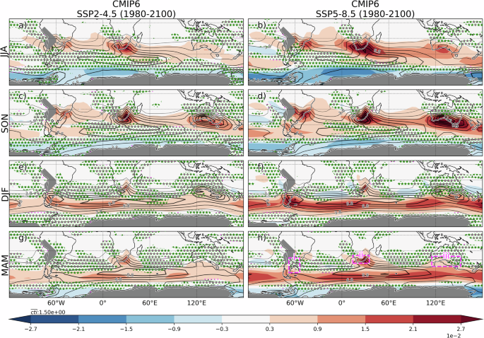
The dynamical mechanisms underlying these differences as well as inter-model uncertainties are also investigated. RESULTS FUTURE PROJECTIONS We first assess long-term (1980–2100) trends in

850-hPa subweekly temperature variability (TVAR; see methods) over the SH in 26 models that participate in CMIP6 (Fig. 1). The 850-hPa level is commonly used to analyze processes driving

temperature variability and trends11,14,27. Important TVAR amplifications are projected to affect midlatitude SH landmasses. The amplification is especially large over South Africa in

June-July-August (JJA) and SON, Australia in SON, and South America in JJA, SON, and DJF, representing TVAR amplifications around its climatological maxima. These amplifications are notably

larger in the most pessimistic scenario (SSP5-8.5) compared to a scenario representing the stabilization of global warming (SSP2-4.5). Even in the latter, the aforementioned trends are

statistically significant as supported by a remarkable agreement among the diverse models. The differences between the two scenarios are found primarily in the amplitude of trends rather

than in their spatial distribution. These trends generally agree with those projected by previous model generations for similar temperature variance metrics11,14. Fig. 2 summarizes the

evolution of TVAR over South America, South Africa, and Australia (see Fig. 1 for their boundaries). Overall, the long-term evolution of TVAR projected under the SSP2-4.5 and SSP5-8.5

scenarios tend to be similar, except for South Africa in JJA and SON and for Australia in SON, where SSP5-8.5 begins to show a markedly larger amplification after ~2049, although its

multi-model mean remains within the inter-model spread of SSP2-4.5. CONTRASTING RECENT TRENDS IN SIMULATIONS AND REANALYSES We then compare the spatial distribution of TVAR trends between

reanalyses and CMIP6 models for 1980–2022 (Fig. 3). TVAR trends in reanalyses are spatially inhomogeneous in the SH15. In the SH extratropics, both positive and negative trends are observed,

although positive trends prevail overall, especially in the mid-to-high latitudes. Over SH landmasses, robust positive trends are found over South Africa and Australia in SON as well as

over South America in DJF and March-April-May (MAM), corresponding to local amplifications of climatological maxima of TVAR. In contrast, the CMIP6 multi-model mean depicts weaker and more

spatially homogeneous changes that are structurally similar, but weaker than long-term trends (Fig. 1). This is likely due to the cancellation of internal variability that affects the

regional scale temperatures28 in the multi-model mean. Still, they are nonetheless not completely homogeneous throughout the SH, suggesting that it can be vital in climate models to

adequately represent stationary waves giving rise to these regional asymmetries and their evolution under anthropogenic forcing for accurate attribution and projection of subweekly

temperature variability. In JJA, the models simulate a tendency for TVAR trends to amplify equatorward of the climatological maximum and decrease poleward over the Atlantic and Indian Ocean

sectors. This is an indication of an overall equatorward shift of the TVAR maxima that affects South Africa. Over Australia and South Africa in SON, by contrast, the simulated amplification

is collocated with the climatological local maxima in TVAR along the southern coasts of both sectors. In DJF, TVAR is simulated to amplify poleward and weaken equatorward of the SH-wide

climatological maxima, similar to the projected change in EKE in CMIP5 models9, indicative of its poleward shift. Although overall the spatial distribution is not similar to that of

reanalyses, an amplification is also simulated over South America in all seasons. Over the satellite era (1979–2022), we observe relatively similar TVAR evolution in South America between

the reanalyses and models, especially in JJA and SON (Fig. 2). Over South Africa, the reanalyses show generally larger TVAR than the model average for all seasons except DJF. Reanalyzed and

simulated evolutions of TVAR in Australia are comparatively more similar, especially in JJA and MAM. In the AMIP simulations where observed sea surface temperature (SST) and sea ice

concentration are imposed (1979–2014), as opposed to freely evolving in the historical, SSP2-4.5, and SSP5-8.5 simulations, some of the model-reanalysis discrepancies in TVAR are reduced.

This is especially obvious for South Africa in JJA and MAM. However, the mitigation is insufficient, and over some sectors and seasons, such as in DJF over South America, it results in a

slightly larger discrepancy from reanalysis compared to coupled simulations. Prior to the introduction of satellite observations into reanalysis data assimilation in 1979, some of the

largest discrepancies between reanalyses and models are observed. During that period, TVAR tends to be larger in the models in almost all seasons and locations except South Africa and

Australia in JJA and MAM. The ability of reanalyses to adequately represent TVAR is most likely hindered during this pre-satellite era due to the reduced availability of upper-air

observations as observational constraints. We note however that surface-input reanalyses that do not assimilate upper-air observations (20CRv2c29, 20CRv330, ERA-20C31) depict an evolution of

TVAR that is reasonably consistent with full-input reanalyses both before and after 197915. This result suggests that surface observations could have mostly constrained 850-hPa temperature

over SH landmasses and therefore that the evolution of TVAR before 1979 may be trustable to some extent. The long-term evolution of TVAR was also shown to be broadly consistent with gridded

surface temperature observations from the Berkeley Earth dataset32. Nonetheless, we hereafter focus on the satellite era for further comparisons to benefit from enhanced observational

constraints. Uncertainties in trends cannot be inferred from Fig. 2 alone. To this end, a more detailed analysis of the TVAR trends follows in Fig. 4. Trends in reanalyses over the 1980–2022

period are clearly larger than simulation averages in Australia in JJA, South Africa in SON, and South America in DJF. We note that if considering the 1970–2022 period, reanalyzed trends

are also significantly larger than simulation averages in South Africa in JJA (not shown; cf. Fig. 2). The reanalyzed trends are within the large spread in trends simulated among the

individual CMIP6 models, which could result from different model physics and/or internal variabilities. For other sectors and seasons some positive or negative differences are also found but

still within the spread among the CMIP6 models. Whereas not all models agree concerning TVAR trends over the 1980–2022 period due to the low signal-to-noise ratio, they almost unanimously

predict positive trends over 1980–2100 to affect South Africa in all seasons except DJF, and Australia in JJA and SON. We note that the CMIP6 models agree less concerning future trends

projected to affect South America. In almost all seasons and locations, TVAR trends in reanalyses are included within the large spread among members of the MPI-ESM1-2-LR large ensemble33,

indicating that internal climatic variability can explain the difference between reanalyses and simulated forced changes, in contrast to the model deficiency previously speculated in the

case of EKE6. An exception is found for South Africa in SON when some of the reanalyses evaluated present larger trends compared to the most extreme ensemble member, suggesting that some

model bias is partly contributing to the differences between models and reanalyses. Comparing trends in reanalyses to trends in the MPI-ESM1-2-LR large ensemble from which the ensemble mean

is removed (Supplementary Fig. 1), we observe that the earlier rise above the 95th percentile of ensemble trends in South America in DJF and Australia in JJA, suggesting that these

amplifications are emerging out of the range that can occur by internal variability alone. The trend is also above the 95th percentile in South Africa in SON, but because of the potential

model discrepancy as mentioned above, the emergence is inconclusive. Supplementary Fig. 2 shows the same analysis repeated for the 1980–2014 period to allow comparison with AMIP experiments.

Differences between reanalyses and the historical simulations are generally similar to those found over 1980–2022. A notable exception is found over Australia in SON when the model

difference with respect to reanalyses becomes negative over 1980–2022, as opposed to 1980–2014, due to the prominent amplification of TVAR in the reanalyses over the past decade (Fig. 2)

that has amplified the trend. We also notice that prescribing SST in the AMIP simulations tends to, but not always, reduce differences in trends. For example, an improvement is noted over

South America in SON, while the difference is exacerbated over South Africa in SON and MAM. Thus, SST variability does not seem to be a significant factor in resolving discrepancies between

simulations and reanalyses. ROLE OF BAROCLINIC PROCESSES An explanation for the discrepancies in TVAR trends between the reanalyses and CMIP6 multi-model mean is sought in the dominant

generation term of temperature variability (Fhoriz) which describes how TVAR is generated by subweekly horizontal advective fluxes of heat that are against the seasonal-mean temperature

gradient (see Methods). The efficiency of the meridional component of TVAR generation \(({F}_{y}^{{eff}}\); Fig. 5) is substantially larger than its zonal counterpart \(({F}_{x}^{{eff}}\);

Supplementary Fig. 3) and as a result is responsible for most of TVAR generation. \({F}_{y}^{{eff}}\) is typically larger in the vicinity of midlatitude land masses such as the eastern coast

of South America and just south of South Africa and Australia, which correspond to sectors of stronger temperature gradients (Supplementary Fig. 4) associated with the land-sea temperature

contrasts. These are also sectors where the correlation between \(-v\mbox{'}\) and \(T\mbox{'}\) tends to exhibit local maxima, denoting optimal eddy structure for the production

of meridional heat fluxes (Supplementary Fig. 5). The magnitude and spatial distribution of these climatological properties are similar between reanalyses and CMIP6 models. Figure 5 however

illustrates a sharp contrast in \({F}_{y}^{{eff}}\) trends between reanalyses and simulations. Whereas both show prominent amplifications of \({F}_{y}^{{eff}}\) over sectors of positive TVAR

trends (comparing with Fig. 3), the CMIP6 models exhibit more moderate trends on average. Like TVAR trends, trends in \({F}_{y}^{{eff}}\) are typically within the wide range of trends among

the models, except for South Africa in SON and MAM when the positive trend is almost three times larger than the simulation average and for South America in MAM when the trends are opposite

(Supplementary Fig. 6). \({F}_{x}^{{eff}}\), although generally weaker, plays a nonnegligible role over the eastern coasts of South Africa and South America (Supplementary Fig. 3). We find

that the differences in \({F}_{y}^{{eff}}\) between the reanalyses and CMIP6 models as well as their spatial distributions are strongly associated with trends in the regional temperature

gradients (Supplementary Fig. 4), confirming the role of the background temperature gradient in setting TVAR trends11,14. But there is an additional contribution from changes in the

correlation between \(v\mbox{'}\) and \(T\mbox{'}\) that describe the eddies’ effectiveness at producing heat fluxes (Supplementary Fig. 5). Trends in the latter are substantially

more prominent in reanalyses compared to CMIP6 models. Simulated long-term trends (1980–2100) in these efficiencies exhibit overall similar geographical distribution to their historical

counterpart (not shown). As further evidence of the role of \({F}_{y}^{{eff}}\), we find that the inter-model differences in TVAR trends are strongly linked to the magnitude of

\({F}_{y}^{{eff}}\) in the vicinity of the land mass sectors examined (Fig. 6). Inter-model correlations can reach up to ~0.6–0.8, especially near South Africa (SON) and Australia (SON) and

South America (DJF). This relationship is not expected to be limited to the land mass sectors of TVAR trends as TVAR is redistributed horizontally by the climatological mean-flow advection

which is typically eastward. Another factor explaining nonlocal correlations is that inter-model diversity in TVAR trends are organized in broader patterns. For example, TVAR trend

differences over South Africa (SON) are linked with TVAR trend differences that span a large portion of SH mid-latitudes and subtropics indicating that local diversity is associated with

broader inter-model differences in the large-scale circulation. Similar correlation patterns are found in temperature gradients, further highlighting the importance of trends in the

broader-scale thermal structure of the atmosphere (Supplementary Fig. 7) for uncertainties in temperature variability. DISCUSSION Given the impact of changing lower-tropospheric temperature

variability on the occurrence of weather extremes16, it seems crucial to further improve its representation in climate models. The large differences between reanalyzed and simulated mean

TVAR trends over some sectors, like the differences in EKE6, may be interpreted as a deficit in the representation of synoptic variability in climate models. The reanalyzed TVAR trends

assessed for recent decades are nevertheless within the inter-model spread that arises from differences in model physics and internal variability, as also suggested by the MPI-ESM1-2-LR

large ensemble33 where the ensemble spread results from internal variability alone. It is thus possible that the discrepancies between the reanalyses and CMIP6 ensemble mean originate from

internal variability that is present in reanalyses but largely averaged out of the model ensemble mean. These findings, therefore, do not undermine the general capability of CMIP6 models to

project future TVAR changes. The range of possible future outcomes may be narrowed in future work by considering the external forcing response of stationary waves, which lead to spatial

inhomogeneities in future changes in the background temperature gradient, and the strength of synoptic eddies’ feedback to these mean flow changes. This approach is supported by the

significant role of temperature anomaly generation efficiency in inter-model uncertainty. If the discrepancy between reanalyses and CMIP6 models is indeed due to internal variability that

has accelerated the rise in TVAR in the recent reanalysis record, we may expect a slowdown, or even a temporary reversal of the trends in the future, akin to the global warming “hiatus”,

which temporarily paused the warming in the early 2000s34,35. This is supported by the large MPI-ESM1-2-LR ensemble whose members with the largest amplification over 1980–2020 show signs of

a slowing or even a reversing of trends in the subsequent decades depending on the location and season (Supplementary Fig. 8). Since ocean-atmosphere coupling was found to be a key factor in

the future poleward shift of the summertime storm track9, we briefly assessed whether the representation of oceanic variability could be a source of model bias. While the AMIP simulations

(1980–2014) can reduce biases in the basic state and trends in some instances, their influence on trends, as well as their discrepancies from reanalyses, is inconsistent across seasons and

sectors. These inconsistencies may stem from internal variability that leads to a weak signal-to-noise ratio when assessing trends over such a short period. Notwithstanding the discrepancies

between the reanalyses and CMIP6 models, we find that all CMIP6 models project important positive TVAR trends (1980–2100) affecting South Africa and Australia in JJA and SON (Figs. 1 and

4). The largest projected increases in South Africa occur in JJA and represent a TVAR amplification of 2.50 ± 0.53% per decade (relative to 1980–2014) in the SSP2-4.5 scenario which may

represent the most likely outcome36, or 4.59 ± 0.97% in what may be the worst case scenario (SSP5-8.5). For Australia, the projected trends are markedly larger in SON with 1.38 ± 0.21% and

2.58 ± 0.40% increases per decade in SSP2-4.5 and SSP5-8.5, respectively. If proven accurate, these sectors should prepare themselves for a substantial increase in subweekly temperature

variability along with profound socioeconomic impacts. Finally, contrasting TVAR trends to EKE trends (Supplementary Figs. 9 and 10), we observe that they do not always agree. For instance,

the SON TVAR amplification over Australia in the reanalyses is accompanied by a decrease in EKE in its vicinity both at 250 and 850 hPa. There is also a general lack of agreement between the

patterns of TVAR and EKE trends in CMIP6 models. This decoupling between near-surface temperature variance and EKE indicates that conventional storm-track metrics based on winds alone are

not appropriate to assess surface impacts, at least concerning the potential impact on heat extremes. Instead, a direct assessment of lower-tropospheric variability is advised based on this

study. METHODS DATA Atmospheric data from reanalyses are used as an approximation of the past state of atmospheric circulation. The Climate Forecast System Reanalysis version 1 (CFSR37) and

version 2 (CFSv238) are combined into a single dataset at their transition between December 2010 and January 2011. Other datasets include the ECMWF Reanalysis v5 (ERA539), the Japanese

55-year Reanalysis (JRA-5540), and the Modern-Era Retrospective analysis for Research and Applications, Version 2 (MERRA-241). Details about their models and data assimilation techniques

have been compiled as part of the S-RIP project42. Climate model projections are obtained from 26 models participating in the CMIP6 project26: ACCESS-CM2, ACCESS-ESM1-5, CAMS-CSM1-0,

CESM2-WACCM, CMCC-CM2-SR5, CNRM-CM6-1, CNRM-CM6-1-HR, CNRM-ESM2-1, CanESM5, EC-Earth3, EC-Earth3-CC, EC-Earth3-Veg, EC-Earth3-Veg-LR, FGOALS-g3, GFDL-CM4, HadGEM3-GC31-LL, INM-CM4-8,

INM-CM5-0, IPSL-CM6A-LR, MIROC-ES2L, MIROC6, MPI-ESM1-2-HR, MPI-ESM1-2-LR, MRI-ESM2-0, NESM3, NorESM2-LM. Model integrations forced by the historical, Shared Socioeconomic Pathway scenario

2-4.5 (SSP2-4.5), and Shared Socioeconomic Pathway scenario 5-8.5 (SSP5-8.5) are investigated. To assess long-term trends, the historical (before 2014) and SSP (after 2015) scenarios are

combined. AMIP-type experiments in which SST is prescribed are also considered. The first ensemble member of each model (i.e., ‘r1i1p1’) is used in this study except for MPI-ESM1-2-LR33 for

which we use 30 ensemble members to assess uncertainties associated with internal climate variability. MPI-ESM1-2-LR is chosen for the large ensemble analysis because it provides the largest

number of ensemble members for which daily data is available for both historical and future climate scenarios. We note that MPI-ESM1-2-LR is not necessarily the model that shows the best

agreement with respect to reanalysis data. Like many other models, differences are improved or worsened compared to the CMIP6 model mean depending on location and season. Similar results are

obtained with the CanESM543 large ensemble for the period 1980–2014 (not shown) but the analysis cannot be extended to 1980–2022 due to the limited number of ensemble members for which

daily data is available for future climate scenarios. Variables analyzed include temperature (\(T\)), pressure velocity (\({\rm{\omega }}\)), and the zonal and meridional wind components

(\(u\) and \(v\), respectively). Daily averages are used. SUBWEEKLY TEMPERATURE VARIABILITY AND ITS LEADING SOURCES AND SINKS By decomposing temperature and winds into the different

timescales they are composed of (e.g., \(T=\overline{T}+T^{\prime} +T^{\prime\prime}\), where the overline, ′, and ″ denote the seasonal mean, subweekly, and subseasonal time scales,

respectively), substituting these components into the atmospheric thermodynamic equation, and then multiplying by \(T^{\prime}\), we obtain an equation expressing the generation and

dissipation of subweekly temperature variability (\(\overline{{{T}^{{\prime} }}^{2}}\) or TVAR): $$\frac{\partial \overline{T^{{\prime} 2}}}{\partial t}=\underbrace{-2\overline{{T}^{{\prime}

}{\bf{v}}^{{\prime} }}\cdot \nabla \overline{T}}_{{F}_{{horiz}}}\underbrace{+2\overline{{T}^{{\prime} }{{\omega }}^{{\prime} }}\left(\frac{R\overline{T}}{{c}_{p}p}-\frac{\partial

\overline{T}}{\partial p}\right)}_{{F}_{{vert}}}+\chi$$ (1) In Eq. 1, only the leading generation and dissipation terms are retained. They are the generation by horizontal wind (1st RHS

term, or Fhoriz) and vertical wind (2nd RHS term, or Fvert). \(\chi\) includes interactions between the subweekly and subseasonal time scales, advection by the seasonal-mean winds which

redistribute TVAR spatially but do not act as overall sources/sinks, diabatic processes, and in the case of reanalysis data, inconsistencies introduced by data assimilation (or analysis

increment). Subweekly variability is here extracted through a 10-day high-pass filter (denoted with primes). By design, the filter allows oscillations with periods up to ~7 days to fully

pass through while oscillations with a 10-day period are damped by ½. Fhoriz and Fvert are considered separately because of the different processes they represent from the perspective of

atmospheric energetics44,45. While both Fhoriz and Fvert are linked to the conversion of available potential energy (APE) from the seasonal-mean horizontal temperature gradient to subweekly

eddies, Fvert receives an additional contribution from the conversion of eddy APE (~TVAR) to EKE. In fact, Fvert is primarily influenced by the latter. In agreement with the typical flows of

energy46, TVAR is usually generated by Fhoriz and dissipated by Fvert15. In this work, we consider only the impact of the source term Fhoriz. Like TVAR, Fhoriz is a function of the product

of eddy terms. Because of this, the amplification of subweekly variability can both amplify TVAR and Fhoriz, thus obscuring the underlying source of the amplification. In this context, it is

more informative to assess changes in the efficiency of energy conversion relative to eddy amplitude. To assess this efficiency, we here scale Fhoriz by the typical magnitude of wind and

temperature variations to obtain $${F}_{y}^{{eff}}=-2\left(\overline{T^{\prime} v^{\prime} }/\sqrt{\overline{{T^{\prime} }^{2}}\,\overline{{v^{\prime} }^{2}}}\right)\partial

\overline{T}/\partial y$$ (2) for the meridional component of Fhoriz efficiency and $${F}_{x}^{{eff}}=-2\left(\overline{T^{\prime} u^{\prime} }/\sqrt{\overline{{T^{\prime}

}^{2}}\,\overline{{u^{\prime} }^{2}}}\right)\partial \overline{T}/\partial x$$ (3) for its zonal component. We note that with such scaling, the eddy terms now describe the correlation

between wind and temperature fluctuations rather than their covariance. Their correlation is determined by the structure of subweekly eddies that will influence, via their horizontal

motions, how wind and temperature fluctuations are synchronized in time. It is a measure for baroclinic eddy growth that generates subweekly variability in the midlatitudes to have

westward-tilting structures with height, which is equivalent to negatively correlated \(v^{\prime}\) and \(T^{\prime}\) in the SH thus producing poleward heat fluxes against the equatorward

background temperature gradient. We note that the efficiency defined here differs from the efficiency in the energetics framework47,48,49 where the source and sink terms are normalized by

the total energy (EKE + EAPE). In addition to TVAR, we also briefly investigate trends in EKE defined as $${EKE}=\frac{\overline{{{u}^{{\prime} }}^{2}}+\overline{{{v}^{{\prime} }}^{2}}}{2}$$

(4) in Supplementary Figs. 9 and 10. These diagnostics are assessed independently in each reanalysis, model, and ensemble member before assessing the ensemble means. When reported as area

averages, these diagnostics are averaged over the grid points located above the land masses included in each sector illustrated in Figs. 1, 3, and 5. DATA AVAILABILITY JRA-55, CFSR, and

CFSv2 data were obtained from the research data archive (https://rda.ucar.edu/). MERRA-2 was obtained from the NASA Goddard Earth Sciences Data and Information Services Center

(https://disc.gsfc.nasa.gov/datasets?project=MERRA-2) and ERA5 was obtained from the climate data store (https://doi.org/10.24381/cds.bd0915c6). CMIP6 model data was obtained from the Earth

System Grid Federation (e.g., https://esgf-node.llnl.gov/projects/cmip6/). CODE AVAILABILITY Code can be provided upon request. REFERENCES * Nakamura, H., Sampe, T., Tanimoto, Y. &

Shimpo, A. Observed associations among storm tracks, jet streams and midlatitude oceanic fronts. _Geophys. Monogr._ 147, 329–345 (2013). Article  Google Scholar  * Hoskins, B. J. &

Hodges, K. I. A new perspective on Southern Hemisphere storm tracks. _J. Clim._ 18, 4108–4129 (2005). Article  Google Scholar  * Nakamura, H. & Shimpo, A. Seasonal variations in the

Southern Hemisphere storm tracks and jet streams as revealed in a reanalysis dataset. _J. Clim._ 17, 1828–1844 (2004). Article  Google Scholar  * O’Gorman, P. A. Understanding the varied

response of the extratropical storm tracks to climate change. _Proc. Natl Acad. Sci. USA_ 107, 19176–19180 (2010). Article  Google Scholar  * Shaw, T. A. et al. Storm track processes and the

opposing influences of climate change. _Nat. Geosci._ 9, 656–664 (2016). Article  CAS  Google Scholar  * Chemke, R., Ming, Y. & Yuval, J. The intensification of winter mid-latitude

storm tracks in the Southern Hemisphere. _Nat. Clim. Chang._ 12, 553–557 (2022). Article  Google Scholar  * Harvey, B. J., Shaffrey, L. C. & Woollings, T. J. Equator-to-pole temperature

differences and the extra-tropical storm track responses of the CMIP5 climate models. _Clim. Dyn._ 43, 1171–1182 (2014). Article  Google Scholar  * Lehmann, J., Coumou, D., Frieler, K.,

Eliseev, A. V. & Levermann, A. Future changes in extratropical storm tracks and baroclinicity under climate change. _Environ. Res. Lett._ 9, 084002 (2014). Article  Google Scholar  *

Chemke, R. The future poleward shift of Southern Hemisphere summer mid-latitude storm tracks stems from ocean coupling. _Nat. Commun._ 13, 1730 (2022). Article  CAS  Google Scholar  * Chang,

E. K. M., Guo, Y. & Xia, X. CMIP5 multimodel ensemble projection of storm track change under global warming. _J. Geophys. Res. Atmos._ 117, 1–19 (2012). Article  Google Scholar  *

Tamarin-Brodsky, T., Hodges, K., Hoskins, B. J. & Shepherd, T. G. A dynamical perspective on atmospheric temperature variability and its response to climate change. _J. Clim._ 32,

1707–1724 (2019). Article  Google Scholar  * Röthlisberger, M. & Papritz, L. A global quantification of the physical processes leading to near‐surface cold extremes. _Geophys. Res.

Lett._ 50, 1–10 (2023). Article  Google Scholar  * Holmes, C. R., Woollings, T., Hawkins, E. & de Vries, H. Robust future changes in temperature variability under greenhouse gas forcing

and the relationship with thermal advection. _J. Clim._ 29, 2221–2236 (2016). Article  Google Scholar  * Schneider, T., Bischoff, T. & Płotka, H. Physics of changes in synoptic

midlatitude temperature variability. _J. Clim._ 28, 2312–2331 (2015). Article  Google Scholar  * Martineau, P., Behera, S. K., Nonaka, M., Nakamura, H. & Kosaka, Y. Seasonally dependent

increases in subweekly temperature variability over Southern Hemisphere landmasses detected in multiple reanalyses. _Weather Clim. Dyn._ 5, 1–15 (2024). Article  Google Scholar  * Simolo, C.

& Corti, S. Quantifying the role of variability in future intensification of heat extremes. _Nat. Commun._ 13, 7930 (2022). Article  CAS  Google Scholar  * Schär, C. et al. The role of

increasing temperature variability in European summer heatwaves. _Nature_ 427, 332–336 (2004). Article  Google Scholar  * Yin, J. H. A consistent poleward shift of the storm tracks in

simulations of 21st century climate. _Geophys. Res. Lett._ 32, 1–4 (2005). Article  Google Scholar  * Vallis, G. K., Zurita‐Gotor, P., Cairns, C. & Kidston, J. Response of the

large‐scale structure of the atmosphere to global warming. _Q. J. R. Meteorol. Soc._ 141, 1479–1501 (2015). Article  Google Scholar  * Butler, A. H., Thompson, D. W. J. & Heikes, R. The

steady-state atmospheric circulation response to climate change–like thermal forcings in a simple general circulation model. _J. Clim._ 23, 3474–3496 (2010). Article  Google Scholar  * Son,

S.-W. & Lee, S. The response of westerly jets to thermal driving in a primitive equation model. _J. Atmos. Sci._ 62, 3741–3757 (2005). Article  Google Scholar  * Wu, Y., Ting, M.,

Seager, R., Huang, H.-P. & Cane, M. A. Changes in storm tracks and energy transports in a warmer climate simulated by the GFDL CM2.1 model. _Clim. Dyn._ 37, 53–72 (2011). Article  Google

Scholar  * Lorenz, D. J. & DeWeaver, E. T. Tropopause height and zonal wind response to global warming in the IPCC scenario integrations. _J. Geophys. Res. Atmos._ 112, 1–11 (2007).

Article  Google Scholar  * Chen, G. & Held, I. M. Phase speed spectra and the recent poleward shift of Southern Hemisphere surface westerlies. _Geophys. Res. Lett._ 34, L21805 (2007).

Article  Google Scholar  * Lim, E.-P. & Simmonds, I. Effect of tropospheric temperature change on the zonal mean circulation and SH winter extratropical cyclones. _Clim. Dyn._ 33, 19–32

(2009). Article  Google Scholar  * Eyring, V. et al. Overview of the Coupled Model Intercomparison Project Phase 6 (CMIP6) experimental design and organisation. _Geosci. Model Dev. Discuss._

8, 10539–10583 (2016). Google Scholar  * Garfinkel, C. I. & Harnik, N. The Non-Gaussianity and spatial asymmetry of temperature extremes relative to the storm track: the role of

horizontal advection. _J. Clim._ 30, 445–464 (2017). Article  Google Scholar  * Arias, P. A. et al. Technical Summary. in _Climate Change 2021 – The Physical Science Basis_ 35–144 (Cambridge

University Press, 2023). https://doi.org/10.1017/9781009157896.002. * Compo, G. P. et al. The Twentieth Century Reanalysis Project. _Q. J. R. Meteorol. Soc._ 137, 1–28 (2011). Article 

Google Scholar  * Slivinski, L. C. et al. Towards a more reliable historical reanalysis: Improvements for version 3 of the Twentieth Century Reanalysis system. _Q. J. R. Meteorol. Soc._ 145,

2876–2908 (2019). Article  Google Scholar  * Poli, P. et al. ERA-20C: an atmospheric reanalysis of the twentieth century. _J. Clim._ 29, 4083–4097 (2016). Article  Google Scholar  * Rohde,

R. A. & Hausfather, Z. The Berkeley earth land/ocean temperature record. _Earth Syst. Sci. Data_ 12, 3469–3479 (2020). Article  Google Scholar  * Olonscheck, D. et al. The New Max Planck

Institute Grand Ensemble With CMIP6 Forcing and High‐Frequency Model Output. _J. Adv. Model. Earth Syst._ 15, 1–21 (2023). Article  Google Scholar  * Kosaka, Y. & Xie, S.-P. The

tropical Pacific as a key pacemaker of the variable rates of global warming. _Nat. Geosci._ 9, 669–673 (2016). Article  CAS  Google Scholar  * Fyfe, J. C. et al. Making sense of the

early-2000s warming slowdown. _Nat. Clim. Chang._ 6, 224–228 (2016). Article  Google Scholar  * Hausfather, Z. & Peters, G. P. Emissions – the ‘business as usual’ story is misleading.

_Nature_ 577, 618–620 (2020). Article  CAS  Google Scholar  * Saha, S. et al. The NCEP climate forecast system reanalysis. _Bull. Am. Meteorol. Soc._ 91, 1015–1058 (2010). Article  Google

Scholar  * Saha, S. et al. The NCEP Climate Forecast System Version 2. _J. Clim._ 27, 2185–2208 (2014). Article  Google Scholar  * Hersbach, H. et al. The ERA5 global reanalysis. _Q. J. R.

Meteorol. Soc._ 146, 1999–2049 (2020). Article  Google Scholar  * Kobayashi, S. et al. The JRA-55 reanalysis: general specifications and basic characteristics. _J. Meteorol. Soc. Jpn. Ser.

II_ 93, 5–48 (2015). Article  Google Scholar  * Gelaro, R. et al. The Modern-Era Retrospective Analysis for Research and Applications, Version 2 (MERRA-2). _J. Clim._ 30, 5419–5454 (2017).

Article  Google Scholar  * Fujiwara, M. et al. Introduction to the SPARC Reanalysis Intercomparison Project (S-RIP) and overview of the reanalysis systems. _Atmos. Chem. Phys._ 17, 1417–1452

(2017). Article  CAS  Google Scholar  * Swart, N. C. et al. The Canadian Earth System Model version 5 (CanESM5.0.3). _Geosci. Model Dev._ 12, 4823–4873 (2019). Article  CAS  Google Scholar

  * Lorenz, E. N. Available potential energy and the maintenance of the general circulation. _Tellus_ 7, 157–167 (1955). Article  Google Scholar  * Oort, A. H. On estimates of the

atmospheric energy cycle. _Mon. Weather Rev._ 92, 483–493 (1964). Article  Google Scholar  * Sheng, J. & Derome, J. An observational study of the energy transfer between the seasonal

mean flow and transient eddies. _Tellus A_ 43, 128–144 (1991). Article  Google Scholar  * Kosaka, Y. & Nakamura, H. Structure and dynamics of the summertime Pacific–Japan teleconnection

pattern. _Q. J. R. Meteorol. Soc._ 132, 2009–2030 (2006). Article  Google Scholar  * Tanaka, S., Nishii, K. & Nakamura, H. Vertical structure and energetics of the western pacific

teleconnection pattern. _J. Clim._ 29, 6597–6616 (2016). Article  Google Scholar  * Martineau, P., Nakamura, H., Kosaka, Y. & Yamamoto, A. Importance of a vertically tilting structure

for energizing the North Atlantic Oscillation. _Sci. Rep._ 10, 12671 (2020). Article  CAS  Google Scholar  * Wilks, D. S. The stippling shows statistically significant grid points”: how

research results are routinely overstated and overinterpreted, and what to do about it. _Bull. Am. Meteorol. Soc._ 97, 2263–2273 (2016). Article  Google Scholar  Download references

ACKNOWLEDGEMENTS This study is in part supported by the Japan Society for the Promotion of Science (JSPS) through Grants-in Aid for Scientific Research (JP19H05702, JP19H05703, JP20H01970,

JP22H01292, JP23K22573, and JP24H02223), by the Japanese Ministry of Education, Culture, Sports, Science and Technology (MEXT) through the Arctic Challenge for Sustainability II (ArCS-II;

JPMXD1420318865) and the Advanced Studies of Climate Change Projection (SENTAN; JPMXD0722680395), by the Japan Science and Technology Agency through COI-NEXT (JPMJPF2013), by the Japanese

Ministry of Environment through Environment Research and Technology Development Fund JPMEERF20242001. AUTHOR INFORMATION AUTHORS AND AFFILIATIONS * Application Laboratory, Research Institute

for Value Added Information Generation, Japan Agency for Marine-Earth Science and Technology, Yokohama, Japan Patrick Martineau, Swadhin K. Behera & Masami Nonaka * Research Center for

Advanced Science and Technology, The University of Tokyo, Tokyo, Japan Hisashi Nakamura & Yu Kosaka Authors * Patrick Martineau View author publications You can also search for this

author inPubMed Google Scholar * Hisashi Nakamura View author publications You can also search for this author inPubMed Google Scholar * Yu Kosaka View author publications You can also

search for this author inPubMed Google Scholar * Swadhin K. Behera View author publications You can also search for this author inPubMed Google Scholar * Masami Nonaka View author

publications You can also search for this author inPubMed Google Scholar CONTRIBUTIONS P.M. led and coordinated the various components of the study throughout. All authors (P.M., H.N., Y.K.,

S.B., and M.N.) discussed the results and aided in their interpretation. P.M. took the lead in writing the manuscript. CORRESPONDING AUTHOR Correspondence to Patrick Martineau. ETHICS

DECLARATIONS COMPETING INTERESTS The authors declare no competing interests ADDITIONAL INFORMATION PUBLISHER’S NOTE Springer Nature remains neutral with regard to jurisdictional claims in

published maps and institutional affiliations. SUPPLEMENTARY INFORMATION SUPPLEMENTARY INFORMATION RIGHTS AND PERMISSIONS OPEN ACCESS This article is licensed under a Creative Commons

Attribution-NonCommercial-NoDerivatives 4.0 International License, which permits any non-commercial use, sharing, distribution and reproduction in any medium or format, as long as you give

appropriate credit to the original author(s) and the source, provide a link to the Creative Commons licence, and indicate if you modified the licensed material. You do not have permission

under this licence to share adapted material derived from this article or parts of it. The images or other third party material in this article are included in the article’s Creative Commons

licence, unless indicated otherwise in a credit line to the material. If material is not included in the article’s Creative Commons licence and your intended use is not permitted by

statutory regulation or exceeds the permitted use, you will need to obtain permission directly from the copyright holder. To view a copy of this licence, visit

http://creativecommons.org/licenses/by-nc-nd/4.0/. Reprints and permissions ABOUT THIS ARTICLE CITE THIS ARTICLE Martineau, P., Nakamura, H., Kosaka, Y. _et al._ Seasonal amplification of

subweekly temperature variability over extratropical Southern Hemisphere land masses. _npj Clim Atmos Sci_ 7, 258 (2024). https://doi.org/10.1038/s41612-024-00804-0 Download citation *

Received: 08 May 2024 * Accepted: 09 October 2024 * Published: 25 October 2024 * DOI: https://doi.org/10.1038/s41612-024-00804-0 SHARE THIS ARTICLE Anyone you share the following link with

will be able to read this content: Get shareable link Sorry, a shareable link is not currently available for this article. Copy to clipboard Provided by the Springer Nature SharedIt

content-sharing initiative