Reader TTS

ABSTRACT The Global Warming Potential-star (GWP*) approach is a way to convert the emissions of short-lived climate forcers to CO2-equivalent emissions while maintaining consistency with

temperature outcomes. Here we evaluate the performance of GWP* when it is used to account for non-CO2 gases within the carbon budget framework. We convert methane (CH4) emissions to

CO2-equivalent emissions via GWP* and calculate the temperature through simple climate models. We show that GWP* can accurately convert CH4 emissions to reproduce the temperature until 2100

under a variety of scenarios, including overshoot scenarios, except those with a rapid decline in CH4 emissions. Beyond 2100, however, the use of GWP* can lead to temperature overestimation

since it extends beyond its calibration range. Furthermore, we find that under scenarios designed to achieve identical temperature targets but with varying overshoot profiles, cumulative

CO2-eq budgets (GWP*-basis) generally increase with overshoot length and magnitude. This is driven by the internal dynamics of our model, as characterized by its negative zero-emission

commitment. While the use of GWP* enhances such effects with increasing overshoot length, it exerts opposite effects with increasing overshoot magnitude. SIMILAR CONTENT BEING VIEWED BY

OTHERS QUANTIFYING NON-CO2 CONTRIBUTIONS TO REMAINING CARBON BUDGETS Article Open access 14 October 2021 AN INTEGRATED APPROACH TO QUANTIFYING UNCERTAINTIES IN THE REMAINING CARBON BUDGET

Article Open access 18 January 2021 A MULTI-MODEL ANALYSIS OF LONG-TERM EMISSIONS AND WARMING IMPLICATIONS OF CURRENT MITIGATION EFFORTS Article 22 November 2021 INTRODUCTION Anthropogenic

climate change is caused by emissions of a range of greenhouse gases (GHGs) that widely vary with respect to their radiative efficiency, atmospheric lifetime, and therefore impact on climate

system1. To deal with GHGs of different characteristics on a common scale, the impact of non-CO2 GHG emissions on climate is sometimes expressed in terms of CO2 equivalent (CO2-eq)

emissions. In doing so, the emissions of non-CO2 GHGs are converted to CO2-eq emissions using GHG emission metrics2. The most widely used metric is the 100-year GWP (GWP100), which is

defined as the time-integrated radiative forcing _over_ 100 years following a pulse emission of one ton of a GHG divided by the corresponding quantity of one ton of CO23,4. Similarly, other

metrics often considered are the GWP20 (with a 20-year reference time period) and the 100-year Global Temperature change Potential (GTP100), which is defined as the global temperature change

following a pulse emission of one ton of a GHG _after_ the reference time period of 100 years divided by the corresponding quantity of one ton of CO25. International climate treaties, such

as the Kyoto Protocol and the Paris Agreement, commonly address multiple GHGs with the use of GWP100 to mitigate climate change cost-effectively6,7,8,9,10. However, when GWP100 is used to

aggregate GHG emissions on a common scale of CO2, the temperature impacts of different GHGs are not accurately captured owing to their diverse behavior in the atmosphere. GHGs fall into two

categories: short-lived climate pollutants (SLCPs) and long-lived climate pollutants (LLCPs)11. There have been decades-long efforts to provide a more accurate emission metric in terms of

the consistency with radiative forcing or temperature5,12,13,14,15,16. GWP100 is not a metric that intends to capture the contrasting temperature responses of LLCP and SLCP

emissions2,11,17,18. CO2, an LLCP, once emitted, will largely remain in the atmosphere (the so-called airborne fraction) with slightly declining concentrations for centuries to

millennia19,20,21. The slightly declining concentrations lead to near-stable warming due to the thermal inertia of the ocean22. It is thus possible to relate cumulative CO2 emissions to the

temperature rise in an almost linear fashion through the widely used transient climate response to cumulative emissions (TCRE)23,24. This provides the basis for the ‘remaining carbon budget

approach’, which is usually used for CO2. In contrast, CH4, an SLCP, is mainly removed from the atmosphere due to atmospheric chemistry processes on faster time scales and thus has a smaller

turnover time in this reservoir. It is currently an active research question how to determine the contribution of CH4 and other SLCPs in the “carbon budget” framework25,26,27,28,29. Unlike

CO2, a pulse emission of CH4 or other SLCPs does not result in near-stable warming; a stable warming is the consequence of a sustained or no increase in the rate of CH4 emissions (or other

SLCP emissions). In other words, a one-off emission of CO2 is approximately comparable to a sustained increase in the emission rate of CH4 in terms of the temperature outcome30,31. A new

metric, GWP*, that captures this fundamental relationship has been proposed, allowing an integration of SLCPs into the carbon budget framework16. Starting from the work of Allen et al.15,

the GWP* metric was built by considering a 20-year time interval to assess the rate of changes in SLCP emissions. Cain et al.16 further improved GWP* by incorporating the small

multi-centennial warming effect arising from SLCP emissions, with an additional term representing the “stock” effect (comparable to the behavior of CO2) on top of the term for the “flow”

effect originally proposed. Therefore, GWP* can be defined by combining the effects from the emission itself (stock) and the change in emissions (flow), with the coefficients _s_ and _r_,

respectively, in Eq. (1). CO2-eq emissions (\({E}_{{CO}2e}\)), which are referred to as CO2-warming equivalent emissions when based on GWP* in Cain et al.16, of SLCP emissions can be

calculated as follows: $${E}_{{CO}2e}={{GWP}}_{H}\times \left[r\times \frac{{\triangle E}_{{\rm{SLCP}}}}{\triangle t\,}\times H+s\times {E}_{{SLCP}}\right]$$ (1) Here, the term _∆E__SLCP_

represents the change in the rate of SLCP emissions with respect to the preceding time interval ∆t, whereas _E__SLCP_ is the emission of the SLCP for that year, and _GWP__H_ is the GWP value

of the SLCP over the time horizon _H_. Originally, by fixing the coefficients _r_ and _s_ to 0.75 and 0.25, respectively, it was possible to ensure a good approximation of CH4 impacts on

temperatures over a range of emissions scenarios (RCP2.6, RCP4.5, and RCP6.0) until 210016,28. Subsequently, a further modification was put forward to scale the right-hand side of Eq. (1) to

ensure the forcing equivalency32. Finally, the GWP* equation adopted in the Sixth Assessment Report of the Intergovernmental Panel on Climate Change (IPCC AR6)33,34, which is used in our

analysis, is the following form: $${E}_{{CO}2e}(t)=0.28\times {E}_{100}(t)+4.25\times \left({{E}_{100}(t)-E}_{100}(t-20)\right)$$ (2) \({E}_{100}(t)\) denotes the emissions of an SLCP

multiplied with its GWP100 value. The first and second terms on the right-hand side of Eq. (2) capture the stock and flow effects, respectively, with a much higher weight given on the flow

effects. Equation (2) is a special case of Eq. (1) with the time interval \(\triangle t\) of 20 years (also modified with a scaling factor of 1.13 discussed above). Note that this formula is

based on GWP100 values in Table 8.A.1 of the IPCC AR5. Although GWP* is often referred to as a metric, GWP* is not a single value: it is rather a more elaborated way of applying existing

GWP100 values. In the traditional approach of using GWP100, the value of GWP100 for the non-CO2 GHG of interest (for both SLCPs and LLCPs) is simply multiplied with the non-CO2 GHG emissions

to calculate CO2-eq emissions. In the GWP* approach, however, the value of GWP100 is multiplied with the emissions and the change in the rate of emissions for a non-CO2 GHG (for SLCPs only)

as in Eq. (1). This approach allows for a more accurate translation of the temperature response of SLCP emissions to that of CO2 emissions when calculating CO2-eq emissions. Scenarios that

exceed the 1.5 °C or 2 °C warming target level temporarily (so-called overshoot scenarios), in which temperatures rise and then fall, are becoming increasingly relevant in the face of

inadequate emission reduction commitments in the policy arena. Although GWP* was proposed with the aim of obtaining a more accurate estimate of temperature changes from cumulative CO2-eq

emissions, the performance of GWP* with declining emissions in overshoot scenarios was not fully assessed in IPCC AR635 and, at the moment of writing this manuscript, has yet to be

systematically tested in any peer-reviewed papers. Previous studies have relied either on specifying the non-CO2 warming response for a given scenario and determining the CO2 contribution as

a residual27,36 or on assuming and exploiting a scenario-dependent relationship between cumulative CO2 emissions and non-CO2 climate forcers37. Another recent approach relies on the concept

of CO2 forcing equivalent (CO2-fe) emissions to consider the contributions of non-CO2 climate forcers29,38. However, implications of using GWP* to determine non-CO2 contributions to the

carbon budget for overshoot scenarios have not been systematically explored. This is particularly relevant to pathways achieving the 1.5 °C warming target, as around 90% of the scenarios

considered in the IPCC Special Report on 1.5 °C (SR15) are either overshoot scenarios for the 1.5 °C target or, more generally, peak and decline scenarios39. Similarly, a large majority of

low emissions scenarios developed from Integrated Assessment Models have been peak and decline scenarios22, with more recently developed stabilization scenarios with net-zero CO2 emissions

being an exception40,41. Lastly, given the current emission trajectory and the recent anomalous warming, overshooting the 1.5 °C target level is projected to be imminent42,43. Moreover,

there is a growing interest in the Earth system modeling community to simulate very long-term overshoot scenarios over a few to several centuries (up to 2300); such very long-term overshoot

scenarios are under development in two Horizon Europe projects, RESCUE and OptimESM. GWP* could be considered as a convenient tool to assess the temperature implication of CH4 emissions of

such scenarios. Whereas GWP* may not be originally intended for such use, considering its calibration range to 2100, users of GWP* are not necessarily aware of the limitations associated

with the calibration range clearly. It is therefore useful to assess how well GWP* serves its purpose over multi-century time scales with different lengths and magnitudes of overshoot.

Therefore, in this paper, we aim to tackle the following scientific questions: Does the GWP* metric adequately ensure equivalent temperature responses when it is used to convert SLCP

emissions to CO2-eq emissions under multi-century scenarios with different lengths and magnitudes of temperature overshoot? Can this metric be used to include non-CO2 contributions in the

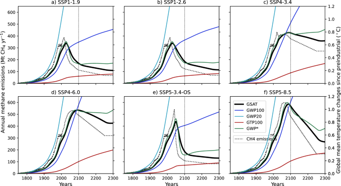
carbon budget approach for overshoot scenarios? RESULTS TESTING THE TEMPERATURE EQUIVALENCY OF GWP* UNDER SSPS We first used a simple Impulse Response Function (IRF) model in IPCC AR51 to

simulate the temperature effect of CH4 emissions under the SSP1-1.9, SSP1-2.6, SSP4-3.4, SSP4-6.0, SSP5-3.4-OS, and SSP5-8.5 scenarios, up to the year 2300. We also calculated the

temperature effect of the CO2-eq emissions that were converted from the CH4 emissions using different emission metrics, such as GWP100 and GWP*. By comparing the two results, we assessed the

extent to which the temperature pathways are maintained or altered with the use of emission metrics in temperature calculations under different SSPs (i.e., “temperature equivalency”). Our

results in Fig. 1 show that GWP100 ensures an imperfect but reasonably good temperature equivalency approximately up to the point of peak CH4 emissions; however, its accuracy decreases

substantially when CH4 emissions decline, a well-known issue with GWP100. It is also shown that GWP100 performs better than GWP20 and GTP100 in terms of the temperature equivalency. GWP20

and GTP100 are illustrative of emphasizing and de-emphasizing, respectively, the temperature effect of CH4 emissions relative to GWP10044,45,46. Thus, the results from GWP20 and GTP100 are

opposite each other, relative to those from GWP100. We further found that GWP* gives a nearly perfect temperature equivalency approximately until the end of the century under the range of

emission scenarios. This result is rather expected, as GWP* is calibrated to do so under the three RCP scenarios. A notable exception is, however, that when CH4 emissions drop sharply, GWP*

overestimates the cooling effect, as shown most evidently under SSP5-3.4-OS (Fig. 1e). This behavior reflects the fact that none of the RCP scenarios used to calibrate GWP* contain a large

overshoot as in SSP5-3.4-OS. It should also be emphasized that, compared to GWP100, GWP* clearly shows superior performances for reproducing the temperature (Table S1). Over the longer run,

however, the temperature equivalency provided by GWP* no longer holds. The cooling effect of CH4 is underestimated or shown even as a slight warming with the use of this metric when CH4

emissions decrease (in all SSPs). From the physical perspective, this is due to the fact that the “stock” parameter, as defined in Cain et al., (2019), emphasize too much the

century-timescale response to earlier methane emission increases, leading to an overestimation of temperatures beyond 2100. These findings are robust since the deviations discussed here are

generally confirmed by two other modeling approaches (Fig. S1). Our findings raise the question regarding whether the use of GWP* could be adequate for accounting for the contribution of CH4

emissions in the carbon budget framework when it is applied for overshoot scenarios, in particular beyond 2100. We then explored the sensitivity of the foregoing results to the parameters

used to define GWP*. We first investigated the sensitivity with respect to the time interval considered between two pulse emissions in the flow term of Eq. 2 (20 years by default, Fig. S2a).

By minimizing the Sum of Squared Errors (SSE) between the temperatures calculated from original CH4 emissions and that from CO2-eq emissions based on the modified GWP* for all the scenarios

in the period 1750-2100, we found the optimal time interval to be 22 years, which is close to the commonly used value of 20 years. Furthermore, we investigated the sensitivity with respect

to the formulation of the flow term in the GWP* equation by substituting the default flow term taking the change in emissions 20 years apart (Eq. 2) with an alternative flow term taking the

_average_ change in emissions over the previous 5, 10, 20, 30, 40 or 50 years (Fig. S2b). Our results show that the use of average change in emissions over the previous 40 years or longer

leads to the best temperature equivalency. We further found that the use of average change in emissions over the previous 40 years yielded a slightly better temperature equivalency than the

use of emissions 20 years apart. We can explain this outcome by the fact that the use of average emissions over 40 years, compared to the use of two end-point emissions 20 years apart, more

closely resembles the exact CO2-eq emissions that precisely reproduce the warming from original CH4 emissions (i.e., the Linear Warming Equivalence emissions)47. However, even when the GWP*

equation is modified in several different ways, the temperature misfit after the rapid drop in CH4 emissions persists (Fig. S3). USING GWP* TO QUANTIFY THE OVERSHOOT CO2-EQ BUDGET Our

analysis based on the SSP scenarios has shown that the temperature equivalency of GWP* can be influenced by the rate of CH4 emission reductions. To gain more insights, we performed a further

analysis based on scenarios with different overshoot lengths and magnitudes. To generate a range of overshoot scenarios, we used the Aggregated Carbon Cycle, Atmospheric Chemistry, and

Climate (ACC2) model9,22,48. ACC2 is a simple climate model49 that resolves many GHGs and aerosols, accounting for primarily important nonlinearities in the global earth system such as CO2

fertilization of the land biosphere, saturation of ocean CO2 uptake under rising atmospheric CO2 concentrations, and climate-carbon cycle feedback. The interaction between CH4 and

tropospheric ozone through the OH chemistry is parameterized in ACC2. The temperature is calculated by using a land-ocean energy balance model coupled with a heat diffusion model (see

“Methods” for details). The simple climate model ACC2 can be further coupled with a climate mitigation module consisting of a set of marginal abatement cost functions9,50 to calculate

least-cost emission pathways for a specified climate target. ACC2 then works as an optimizing climate-economy model, and we took advantage of this model feature to systematically generate

overshoot pathways for our analysis. We also took advantage of the more detailed process representations of ACC2, relative to the IRF model, while simplicity is maintained in ACC2 for

performing sensitivity simulations. We use ACC2 to generate a range of pathways that reach the 1.5 or 2 °C target level after overshoot of varying lengths and magnitudes. We calculate

least-cost emission scenarios to keep the temperature below a target level throughout the simulation period (temperature _stabilization_ pathways). If we apply the temperature target only

after a certain year, the model yields least-cost emission scenarios that lead to temperature _overshoot_ pathways. In this case, the temperature exceeds the target level before that year,

since it is less costly to invest in mitigation efforts later in the cost-effectiveness framework as also pointed out by previous studies51,52. The length and the magnitude of the

temperature overshoot are determined by ACC2’s internal cost minimization reflecting assumptions on the maximum rates of emission abatements and the discounting rate. We varied the target

years between 2060 and 2180 with an interval of 10 years and selected appropriate target years to be tested for each temperature goal (1.5 °C and 2 °C). For each target year, we further

varied the discount rate to 2% and 6%, compared to the original 4% by default, to generate different overshoot magnitudes, while keeping the same overshoot length. Emissions of all climate

forcers other than CO2 and CH4 are assumed to follow SSP1-1.9 and SSP1-2.6 in the case of the 1.5 and 2 °C targets, respectively. For each pathway, we calculated the “overshoot CO2-eq

budget” which is defined as the cumulative net CO2-eq emissions (GtCeq) from 2020 till the year when the temperature stabilizes at or returns to the 1.5 or 2 °C warming target level after

temperature overshoot. The overshoot CO2-eq budget discussed in this paper implicitly assumes that positive and negative emissions can be equally balanced, although the validity of this

assumption will be explored later in this paper. The carbon budget for this time frame is referred to as the threshold return budget elsewhere25,53, but we include non-CO2 contributions in

the threshold return budget using the emission metric approach: GWP* for SLCPs and GWP100 for LLCPs. For the sake of analysis, our overshoot CO2-eq budget considers only CO2 and CH4, unless

stated otherwise, which are our focus but are largely representative of the entire CO2-eq budget because these two gases are usually most important for climate change mitigation. We present

the results calculated from ACC2 emulating IPSL-CM6A-LR in the main paper. Qualitatively similar results can be found from ACC2 emulating other ESMs, as in Figs. S4 and S5 for CNRM-ESM2-1

and MIROC-ES2L. MULTI-GAS OPTIMIZATION EXPERIMENTS We first performed _multi-gas_ optimization experiments (Fig. 2), where CO2 and CH4 emission pathways are optimized simultaneously using

the ACC2 setup to calculate the least-cost pathways, while all other gases and pollutants are assumed to follow SSP1-1.9 and SSP1-2.6 in the case of the 1.5 °C (Fig. 2a, c) and 2 °C target

(Fig. 2b, d), respectively. Panels (a) and (b) of Fig. 2 show the overshoot CO2-eq budget (with CH4 converted via GWP*) for different 1.5 °C and 2 °C stabilization years, respectively, with

ranges of overshoot magnitude and length. For both the 1.5 °C and 2 °C target year simulations, we found that the longer the temperature overshoot is, the larger the overshoot CO2-eq budget

is. Furthermore, for the same overshoot length, the higher the overshoot is, the larger the overshoot CO2-eq budget is (the 2 °C case with the 2060 target year is an exception because the

target lengths and magnitudes are not clearly separated) (Table 1). The increasing total overshoot CO2-eq budget with increasing overshoot lengths and magnitudes reflects both the model

behavior of ACC2 and the conversion of CH4 emissions to CO2-eq emissions via GWP*, which will be disentangled in the analysis presented in the next section. The contribution of CH4 in the

overshoot CO2-eq budget becomes particularly important for 1.5 °C pathways, in which the total overshoot CO2-eq budget is so small that the contribution from CH4 can even determine the sign

of the total overshoot CO2-eq budget. This indicates that how to account for CH4 contributions to the overshoot CO2-eq budget is crucial for mitigation pathways aiming at the 1.5 °C target

level. The overshoot CO2-eq budgets calculated with our default version of ACC2 are generally low because this version of ACC2 was configured to IPSL-CM6A-LR, which exhibits a high climate

sensitivity (Table S4 and Figs. S10 and S11). The overshoot CO2-eq budget is in fact already negative in about a half of the cases for the 1.5 °C target level, specifically for scenarios

with target years in 2090 and 2120. These negative overshoot CO2-eq budgets reflect deep CO2 mitigation that is required to compensate for the limited CH4 mitigation (Fig. S6 for simulations

for the target year of 2120 with three different overshoot profiles), as well as the unmasked warming from decreasing emissions of air pollutants (following SSP1-1.9 for 1.5 °C target

scenarios). In the remaining cases with high and long overshoots, on the other hand, some more emissions are still left in the budget. SINGLE-GAS OPTIMIZATION EXPERIMENTS We further

performed _single-gas_ optimization experiments (Fig. 3). In this case, only the emission pathway of one of the two gases (CO2 or CH4) is optimized to reach the target temperature with

lowest cost, while the emission pathways of all other gases and pollutants are kept at the respective SSP scenario (SSP1-1.9 or SSP1-2.6) corresponding to the target temperature (1.5 or 2 °C

target level). This experiment is useful to isolate the relative contribution of CO2 and CH4 to the overshoot CO2-eq budget. That is, unlike the previous experiments, in which emission

reductions of CO2 and CH4 can be traded to yield a least-cost solution, emission reductions of only one gas can change with varying overshoot lengths and magnitudes in these experiments. As

for Fig. 2, panels a) and b) of Fig. 3 report the overshoot CO2-eq budget calculated for each simulation of the single-gas optimization experiments, for CO2 cumulative emissions and CO2-eq

cumulative emissions (CH4 converted with GWP*), respectively. In the case of CO2-only optimization experiment (Fig. 3a), the longer the temperature overshoot is, the larger the overshoot

CO2-eq budget is. This finding is in contrast to the general belief that the carbon budget is reduced with increasing overshoot lengths54,55. We found qualitatively similar results for the

CH4-only optimization experiment as well (Fig. 3b). Caution must be taken in drawing conclusions from this, as it could be interpreted that a late mitigation is preferred compared to early

mitigation actions. It should be noted that this finding is dependent on model assumptions, such as CO2 fertilization effect (Figure S8), and model characteristics as discussed in the next

section. The results for overshoot magnitudes provide a further insight: the higher the overshoot is for the same overshoot length, the larger the overshoot CO2-eq budget is from the

CO2-only optimization experiment, but the smaller the overshoot CO2-eq budget is from the CH4-only optimization experiment (in most cases). The results of the CO2-only optimization

experiment reflect the dynamic behavior of ACC2 (analyzed in the next section); those of the CH4-only optimization experiment, on the other hand, not only reflect the model’s dynamic

behavior but also the conversion of CH4 emissions to CO2-eq emissions via GWP*. In the analysis that follows, we further delve into this finding separately in the ramp-up and ramp-down

periods of overshoot scenarios. Note that CH4 contributions to the overshoot CO2-eq budget of the CH4-only optimization experiment are higher in the 1.5 °C target case than those in the 2 °C

target case, which appears counterintuitive first since a lower temperature target usually implies stricter emission limits. This phenomenon is due to the higher relative contributions of

the prescribed CO2 baseline scenario to the total radiative forcing in SSP1-2.6 (used for the 2 °C target simulations) compared to those in SSP1-1.9 (used for the 1.5 °C target simulations).

TCRE OF THE RAMP-UP AND RAMP-DOWN PHASES OF OVERSHOOT SCENARIOS To gain insight into how the model’s dynamic behavior influences the overshoot CO2-eq budget in different phases of overshoot

scenarios, we looked into the TCRE separately for the ramp-up and ramp-down phases. We computed TCRE, for each single-gas optimization experiment, as the ratio of the temperature change

over the cumulative CO2-eq emissions for the sum of three gases (CO2, GWP*-weighted CH4, and GWP100-weighted N2O). We distinguish TCRE between the ramp-up (from year 1750 to the year of peak

emissions) and the ramp-down phases (from the year of peak emissions to the year when the temperature target is met after overshoot) as TCRE+ and TCRE−, respectively. The current literature

does not provide sufficient clarity regarding the extent to which the linear relationship between cumulative CO2 emissions and temperature changes holds in case of negative emissions56. As

reported in Chapter 5 of IPCC AR6 WGI, there is no clear agreement among models for the relationship between TCRE+ and TCRE−35. Figure 4 shows the results from both the CO2-only optimization

and CH4-only optimization experiments for the 1.5 °C target. In Fig. 4a, c, cumulative emissions consider only one gas (CO2 or GWP*-weighted CH4), but the warming is calculated from the

emissions of all gases, indicating that the cumulative emissions are not necessarily consistent with the simulated warming. In Fig. 4b, d, on the other hand, cumulative emissions consider

the three major gases, which is thus approximately consistent with the simulated warming, but the effects from individual gases cannot be isolated. The values of TCRE+ and TCRE− (°C/1,000

GtCeq) reported in panels b) and d) represent the mean of all TCRE+ and TCRE− values from the scenarios presented in the panels. The general indication is that TCRE− is larger than TCRE+,

which is consistent with the finding from Fig. 2 and Fig. 3: the longer or higher the temperature overshoot is, the larger the overshoot CO2-eq budget is. An exception is the decreasing

TCRE− with increasing overshoot magnitudes from the CH4-only optimization experiments (Fig. 4d). By taking the average of TCRE− across the scenarios with low, medium, and high overshoot

(i.e., for discount rates of 2%, 4%, and 6%), the TCRE− values are indeed decreasing with increasing overshoot magnitudes, which are 3.1, 2.9, and 2.7, respectively (mean value of 2.9, as

reported in Fig. 4d). This can be confirmed with our earlier finding that the overshoot CO2-eq budget decreases with increasing overshoot magnitudes in the CH4-only optimization experiment

owing to the use of GWP*. The relatively large TCRE− from the CO2-only optimization experiment can be further confirmed with the Zero Emission Commitment (ZEC) parameters of this model.

Following the ZEC Model Intercomparison Project (ZECMIP) framework described in Jones et al.57, we performed the B.1, B.2, and B.3 experiments as in MacDougall et al.58 to compute the ZEC

parameters (Fig. S9). These three experiments use 100-year bell-shaped CO2 emissions of 1000 GtC, 750 GtC, and 2000 GtC, respectively, starting from pre-industrial conditions, aiming to

assess the model-specific climate inertia in the decades after a complete cessation of emissions. We report the estimates of ZEC25, ZEC50, and ZEC90, representing the temperature change

respectively 25, 50, and 90 years after the start of zero emissions. Table 2 shows that all three ZEC parameters are negative for ACC2, which supports the large TCRE− relative to TCRE+. We

further note that the ZEC parameters for different configurations of ACC2 (emulated to CNRM-ESM2-1 and MIROC-ES2L used for sensitivity analyses) also present negative values (Fig. S9). It

should be emphasized that there is generally no consensus for the relationship between TCRE+ and TCRE−, among models, as demonstrated by previous studies54,55,59,60,61,62. The lack of

consensus is also evident from the analysis of 1pct-CO2-cdr idealized experiment56, where MIROC-ES2L and CanESM5 report larger TCRE− than TCRE+ whereas UKESM1-0-LL and ACCESS-ESM1-5 show

smaller TCRE+ than TCRE− (Fig. S12). DISCUSSION This study examined how the emissions of non-CO2 GHGs, in particular CH4, can be accounted for in the overshoot CO2-eq budget framework. A key

requirement for including non-CO2 contributions in the CO2-eq budget framework is to ensure the temperature equivalency. That is, non-CO2 emissions should be converted to CO2-eq emissions

in such a way that the implied temperature outcome remains the same. Recently, the GWP* approach has received attention; however, this approach has not been extensively evaluated for

overshoot scenarios or, more generally, peak and decline scenarios in a long time scale. Our analysis using the SSP scenarios confirmed that GWP* does a reasonably good job of ensuring a

temperature equivalency for a range of pathways up to 2100 when it is used to convert CH4 emissions to CO2-eq emissions. An exception is that when the temperature drops sharply in the

ramp-down phase of overshoot, the use of GWP* leads to an overestimation of cooling. Over a longer time scale up to 2300, when the temperature decreases moderately, the use of GWP* can lead

to an underestimation of cooling or indicate a slight warming instead. These findings are related to the fact that GWP* was tuned to a certain set of pathways up to 2100. Our results indeed

showed that the deviation tends to become more evident after 2100. These findings suggest that GWP* should be cautiously used for scenarios with strong decline in temperatures and/or

longer-term peak and decline scenarios beyond 2100. Nevertheless, GWP* is still far superior to the standard and most widely used metric GWP100 in terms of the temperature equivalency under

all scenarios. We have attempted to improve GWP* by modifying the parameters in the GWP* equation, but this did not result in any substantial improvement in temperature equivalency. It

should be noted that the IRF was used for temperature calculations here in order to be consistent with the underlying methods used to derive metric values in AR5 and the GWP* formula in AR6.

When ACC2 and FaIR are used for temperature calculations, our general findings still hold; however, the quantitative results become different particularly from ACC2, reiterating the fact

that the GWP* formula is model-dependent or reflects certain model assumptions, a point that deserves more attention. Our study further investigated how the overshoot CO2-eq budget for the

1.5 and 2 °C target levels, including the contribution of CH4 based on GWP*, can be affected by the temperature overshoot of varying lengths and magnitudes. We generated a set of scenarios

to reach the representative temperature target levels with overshoot of different lengths and magnitudes through cost-effective calculations of ACC2 configured to several different

state-of-the-art ESMs. Our results generally showed that the overshoot CO2-eq budget increases with the length and magnitude of overshoot, except under CH4-varying scenarios with different

overshoot magnitudes. This finding is mainly related to the model property of ACC2 that it takes larger cumulative CO2 emissions in absolute terms to produce a given amount of warming than

it takes to produce the same amount of cooling in absolute terms. In other words, TCRE+ is smaller than TCRE− in ACC2, which is also consistent with the negative ZEC, found in our analysis

for ACC2. Importantly, this finding is modified by the conversion of CH4 emissions into CO2-eq emissions via GWP*. The application of GWP* on CH4 has an effect of decreasing the apparent

overshoot CO2-eq budget with increasing overshoot magnitudes. To summarize, the use of GWP* to include CH4 in the CO2-eq budget framework in case of overshoot scenarios works in most

scenario until 2100, except for cases with a rapid decline in CH4 emissions. Over a longer run beyond 2100, the use of GWP* can overestimate the warming effect of CH4 emissions and

consequently may lead to an overestimation of CO2-eq budget. It should however be noted that these results depend on the model configuration used for the analysis, requiring further studies

based on different modeling approaches, including uncertainty analyses of Earth system feedbacks. METHODS DESCRIPTION OF THREE REDUCED-COMPLEXITY MODELS Our analysis used three different

reduced-complexity models as follows in the order of increasing complexity: the Impulse Response Function (IRF) model of IPCC AR51, the Finite Amplitude Impulse Response (FaIR) model63,64,

and the Aggregated Carbon Cycle, Atmospheric Chemistry, and Climate (ACC2) Model9,22,48. First, the IRF model is a simplified representation of the atmospheric response to a pulse emission

of CO2. It approximates the fraction of emitted carbon that remains in the atmosphere over time21, to estimate the temperature impact of GHG emissions according to the radiative efficiencies

of the single GHG. The IRF model used in our study is derived from the latest estimates summarized in the IPCC AR5. It is employed to estimate the temperature response of CO2-eq emissions

derived from CH4 using various conversion metrics. Second, the FaIR v1.3 has been extensively used for assessing the temperature impacts of different emissions pathways and mitigation

scenarios16,27,38,65. FaIR has a simple representation of the carbon cycle and accounts for nonlinear feedback such as the temperature and saturation dependency of land and ocean carbon

sinks. The model calculates both CO2 and non-CO2 GHG atmospheric concentrations by tracking their time-integrated airborne fraction from their initial emissions. From concentrations,

Effective Radiative Forcing (ERF) for thirteen forcings, including land-use change, tropospheric and stratospheric O3 as well as other GHG are computed; finally the temperature change is

calculated as the sum of its slow and fast components, representing temperature changes from a response to forcing from the upper ocean and the deep ocean, respectively. Third, ACC2 is a

simple climate-economy model composed of four modules: i) carbon cycle, ii) atmospheric chemistry, iii) physical climate, and iv) economy. The carbon cycle module is made of three ocean

boxes, a coupled atmosphere-mixed layer box, and four land boxes. The physical climate module is the land-ocean energy balance model coupled with the heat diffusion model DOECLIM, which is

used to calculate the temperature response to radiative forcing48. The radiative forcing is calculated for the following direct and indirect climate forcers: CO2, CH4, N2O, O3, SF6, 29

halocarbon species, OH, VOC, CO, NOx, stratospheric H2O, sulfate aerosols, and carbonaceous aerosols (both direct and indirect effects). The changes in CH4 and N2O concentrations are given

as a function of their atmospheric concentrations, the sum of anthropogenic and natural emissions, and their lifetime. ACC2 accounts for nonlinear feedbacks such as the saturation of ocean

CO2 uptake under rising CO2 concentration, CO2 fertilization of the land biosphere, and increasing heterotrophic respiration of the land biosphere with rising temperatures. Furthermore,

uncertain parameters in ACC2 are calibrated with a Bayesian approach13,22. The model is developed in the GAMS programming language and numerically solved using CONOPT3 and CONOPT4, two

nonlinear optimization solvers included in the GAMS software package. When ACC2 is used as a simulator, the first three modules are used to calculate temperature changes based on prescribed

emissions scenarios. On the other hand, when ACC2 is used as an optimizer, all four modules, including the economy module consisting of the marginal abatement cost curves50 for global CO2,

CH4, and N2O emissions, are used to derive least-cost emission pathways for a given climate target. ACC2 has participated in model intercomparison projects21,49 and has been subject to

comparison with other models in other studies66. This model has been applied to analyze pathways to achieve the targets of the Paris Agreement9,22,67 including GHG removal options68. The

performance of ACC2 configured for this paper with three EMSs was benchmarked against other simple climate models under commonly used scenarios RCP2.6 and RCP4.5 in the emission-driven

mode49 (Figs. S10 and S11). CARBON CYCLE PARAMETERS IN ACC2 As in many simple climate and carbon cycle models, a steady state is assumed for the carbon cycle in the preindustrial period69.

In 1750, the preindustrial start year of ACC2, the Net Primary Production (NPP) was assumed to be constant and in balance with the heterotrophic respiration. The perturbation of the NPP and

the resulting changes in heterotrophic respiration are described by the four-reservoir land box model. A change in atmospheric CO2 concentration logarithmically influences the NPP (i.e., CO2

fertilization), the strength of which is scaled with the BETA factor. On the other hand, the heterotrophic respiration is exponentially dependent on the temperature as parameterized through

a Q10 factor, at the rate of which the heterotrophic respiration increases with a temperature increase of 10 °C. The governing equation for each of the four land reservoirs is:

$$\begin{array}{l}{\dot{c}}_{{ter},l}\left(t\right)={A}_{{ter},l}{\tau }_{{ter},l}\left({\bar{f}}_{{NPP}}^{{pre}}+\delta {f}_{{NPP}}\left(t\right)\right)\\\qquad\qquad\quad-\,\frac{1}{{\tau

}_{{ter},l}}\left({\bar{c}}_{{ter},l}^{{pre}}+{c}_{{ter},l}\left(t\right)\right)q\left(t\right){{\rm{with}}\; {\rm{l}}}=[1{{\mbox{-}}}4]\end{array}$$ (3) Here, the first term on the

right-hand side of Eq. (3) represents added carbon to the reservoir _l_: the increase in NPP of year _t_ (\(\delta {f}_{{NPP}}\left(t\right)\)) combined with the preindustrial constant NPP

(\({\bar{f}}_{{NPP}}^{{pre}}\)). \({A}_{{ter},l}\) and \({\tau }_{{ter},l}\) represents the coefficients and the overturning time constants of the IRF describing the temporal evolution of

biomass for each reservoir. The second term represents released carbon from the reservoir _l_: the release of carbon from both preindustrial (\({\bar{c}}_{{ter},l}^{{pre}}\)) and fertilized

storage (\({c}_{{ter},l}\left(t\right)\)), which can be enhanced under warming through \(q\left(t\right)\), the Q10 factor, accounting for climate-carbon cycle feedbacks. Furthermore, the

BETA (\({\beta }_{{NPP}}\)) and Q10 factors used to parameterize the CO2 fertilization effect on photosynthesis and temperature control on heterotrophic respiration, respectively, are

expressed in the two following equations: $$\delta {f}_{{NPP}}\left(t\right)={\bar{f}}_{{NPP}}^{{pre}}{\beta

}_{{NPP}}\mathrm{ln}\left(\frac{{pC}{O}_{2}\left(t\right)}{{pC}{O}_{2}^{{pre}}}\right)$$ (4) $$q\left(t\right)={Q}_{10}\frac{\delta {T}_{{land}-{air}}\left(t\right)}{10}$$ (5) Note that the

BETA factor is a commonly used parameter representing the CO2 fertilization effect (more technically, a scaling parameter expressing the sensitivity of the change in NPP to the logarithmic

change in atmospheric CO2 concentrations) but importantly differs from another commonly used parameter β also representing a quantity including the CO2 fertilization effect (a scaling

parameter expressing the sensitivity of the carbon storage to the change in atmospheric CO2 concentrations, expressed in GtC ppm−1)62,70,71,72. EMULATING ACC2 TO CMIP6 ESMS We emulated ACC2

to five state-of-the-art ESMs (CanESM5, CNRM-ESM2-1, IPSL-CM6A-LR, MIROC-ES2L, and UKESM1-0-LL, see Table S2 for an overview of the ESMs) developed under the Coupled Model Intercomparison

Project 6, CMIP673. The emulation was performed using SSP5-3.4-OS, a high-temperature overshoot scenario combining the high emission SSP5-8.5 scenario until 2040 with strong mitigation

thereafter74. We used the data from the fully-coupled (COU) configuration of ESMs. Our emulation method focuses only on three key parameters: namely, the equilibrium climate sensitivity

(ECS), BETA, and Q10. Overall, three configurations of ACC2 emulating IPSL-CM6A-LR, CNRM-ESM2-1, and MIROC-ES2L have been used for the analysis because relatively large number of scenarios

were obtained from these three configurations for the range of temperature targets and overshoot profiles considered in this study. We first calibrated the ACC2 temperature response with

that of each ESM. By tuning the ECS parameter in ACC2 (Table S3), we determined, for each ESM, the value of ECS which yielded the closest projection to each ESM (Fig. S13 and Table S4).

Then, we tuned BETA and Q10 values to emulate NBP (Table 2). We considered NBP to capture carbon concentration and carbon-climate feedback effects. We adjusted NBP estimates of ACC2 to

correct for a lack of representation of land-use change (LUC) processes in ACC2. That is, LUC emissions data from the Global Carbon Budget75 from 1850 to 2014 and integrated assessment

models (IAM) output from 2015 to 2100 for the SSP5-3.4-OS76,77 were used to make the ACC2 output comparable with ESMs. We identified the best combination of BETA and Q10 values for each ESM,

for which the RMSE of the NBP estimates from ACC2 relative to the NBP from the ESM is minimized. The results of the emulation process are shown in Table S4 and Figs. S14–S17. Our emulation

for ACC2 gives similar or systematically lower ECS values compared to those reported elsewhere78, with an average difference of 0.64 °C. In Fig. S14, NBP from ACC2 with the best combination

of BETA and Q10 values for each ESM is compared with NBP from the respective ESM. Apart from the inter-annual variability, the emulation shows overall a good performance for both the ramp-up

and ramp-down phases. We further evaluated the emulation of IPSL-CM6A-LR with ACC2 by using the optimal combination of ECS, BETA, and Q10 parameters to simulate seven additional scenarios.

Figures S15–S17 show the land carbon uptake, ocean carbon uptake, and temperature evolution from the emulated ACC2 and IPSL-CM6A-LR. The temperature change was reproduced very well overall

for all the SSP scenarios considered. Some over-estimation of ocean carbon uptake, on the other hand, occurred in ACC2 when the ocean carbon uptake declined. This inconsistency may be

related to a faster mixing of carbon from the surface to the deep ocean in simple climate models66. Land carbon uptake showed a significant misfit in the cases of medium to high forcing

scenarios (SSP2-4.5, SSP4-6.0, SSP3-7.0, and SSP5-8.5), which gives >3 °C warming at the end of this century. The largest warming level considered in our analysis using the ranges of

overshoot scenarios (Figs. 2, 3) is approximately 3 °C (or 1 °C overshoot of the 2 °C target level). Thus, the misfit found here does not pose a problem for our application, given the range

of our model application. DATA AVAILABILITY The data used for replicating the analysis and the figures presented in this work can be found in the following GitHub repository:

https://github.com/Matteo-Mastro/GWP_overshoot.git. CODE AVAILABILITY The codes used for replicating the analysis and the figures presented in this work can be found in the following GitHub

repository: https://github.com/Matteo-Mastro/GWP_overshoot.git. REFERENCES * Myhre, G. et al. Anthropogenic and Natural Radiative Forcing. in _Climate Change 2013: The Physical Science

Basis. Contribution of Working Group I to the Fifth Assessment Report of the Intergovernmental Panel on Climate Change_ (Cambridge University Press, Cambridge, United Kingdom and New York,

NY, USA, 2013). * Tanaka, K., Peters, G. P. & Fuglestvedt, J. S. Policy update: multicomponent climate policy: why do emission metrics matter? _Carbon Manag._ 1, 191–197 (2010). Article

  Google Scholar  * Lashof, D. A. & Ahuja, D. R. Relative contributions of greenhouse gas emissions to global warming. _Nature_ 344, 529–531 (1990). Article  CAS  Google Scholar  *

UNFCCC. Common metrics | UNFCCC. https://unfccc.int/process-and-meetings/transparency-and-reporting/methods-for-climate-change-transparency/common-metrics (2023). * Shine, K. P., Berntsen,

T. K., Fuglestvedt, J. S., Skeie, R. B. & Stuber, N. Comparing the climate effect of emissions of short- and long-lived climate agents. _Philos. Trans. R. Soc. A Math. Phys. Eng. Sci._

365, 1903–1914 (2007). Article  CAS  Google Scholar  * Manne, A. S. & Richels, R. G. An alternative approach to establishing trade-offs among greenhouse gases. _Nature_ 410, 675–677

(2001). Article  CAS  Google Scholar  * O’Neill, B. C. Economics, natural science, and the costs of global warming potentials. _Clim. Change_ 58, 251–260 (2003). Article  Google Scholar  *

Tol, R. S. J., Berntsen, T. K., O’Neill, B. C., Fuglestvedt, J. S. & Shine, K. P. A unifying framework for metrics for aggregating the climate effect of different emissions. _Environ.

Res. Lett._ 7, 044006 (2012). Article  Google Scholar  * Tanaka, K., Boucher, O., Ciais, P., Johansson, D. J. A. & Morfeldt, J. Cost-effective implementation of the Paris Agreement using

flexible greenhouse gas metrics. _Sci. Adv._ 7 (2021). * UNFCCC. Report of the Conference of the Parties serving as the meeting of the Parties to the Paris Agreement on the third part of

its first session, held in Katowice from 3 to 14 December 2018. Addendum 2. (2018). * Allen, M. R. et al. Indicate separate contributions of long-lived and short-lived greenhouse gases in

emission targets. _NPJ Clim. Atmos. Sci._ 5, 1–4 (2022). _2022 5:1_. Article  Google Scholar  * Wigley, T. M. L. The Kyoto Protocol: CO2 CH4 and climate implications. _Geophys. Res. Lett._

25, 2285–2288 (1998). Article  CAS  Google Scholar  * Tanaka, K. et al. Evaluating global warming potentials with historical temperature. _Clim. Change_ 96, 443–466 (2009). Article  CAS 

Google Scholar  * Tanaka, K., Johansson, D. J. A., O’Neill, B. C. & Fuglestvedt, J. S. Emission metrics under the 2 °C climate stabilization target. _Clim. Change_ 117, 933–941 (2013).

Article  CAS  Google Scholar  * Allen, M. R. et al. A solution to the misrepresentations of CO2-equivalent emissions of short-lived climate pollutants under ambitious mitigation. _NPJ Clim.

Atmos. Sci._ 1, 1–8 (2018). _2018 1:1_. Article  Google Scholar  * Cain, M. et al. Improved calculation of warming-equivalent emissions for short-lived climate pollutants. _NPJ Clim. Atmos.

Sci._ 2, 1–7 (2019). _2019 2:1_. Article  CAS  Google Scholar  * Fuglestvedt, J. S. et al. Metrics of climate change: assessing radiative forcing and emission indices. _Clim. Change_ 58,

267–331 (2003). Article  Google Scholar  * Pierrehumbert, R. T. Short-lived climate pollution. _Annu. Rev. Earth Planet. Sci._ 42, 341–379 (2014). Article  CAS  Google Scholar  * Archer, D.

et al. Atmospheric lifetime of fossil fuel carbon dioxide. _Annu. Rev. Earth Planet. Sci._ 37, 117–134 (2009). Article  CAS  Google Scholar  * Eby, M. et al. Lifetime of anthropogenic

climate change: millennial time scales of potential CO2 and surface temperature perturbations. _J. Clim._ 22, 2501–2511 (2009). Article  Google Scholar  * Joos, F. et al. CO2 and climate

impulse response functions for metric computation atmospheric chemistry and physics discussions carbon dioxide and climate impulse response functions for the computation of greenhouse gas

metrics: a multi-model analysis. _Atmos. Chem. Phys. Discuss_ 12, 2793–2825 (2013). * Tanaka, K. & O’Neill, B. C. The Paris Agreement zero-emissions goal is not always consistent with

the 1.5 °C and 2 °C temperature targets. _Nat. Clim. Change_ 8, 319–324 (2018). _2018 8:4_. Article  CAS  Google Scholar  * Allen, M. R. et al. Warming caused by cumulative carbon emissions

towards the trillionth tonne. _Nature_ 458, 1163–1166 (2009). Article  CAS  Google Scholar  * Matthews, H. D., Gillett, N. P., Stott, P. A. & Zickfeld, K. The proportionality of global

warming to cumulative carbon emissions. _Nature_ 459, 829–832 (2009). Article  CAS  Google Scholar  * Rogelj, J., Forster, P. M., Kriegler, E., Smith, C. J. & Séférian, R. Estimating and

tracking the remaining carbon budget for stringent climate targets. _Nature_ 571, 335–342 (2019). Article  CAS  Google Scholar  * Damon Matthews, H. et al. An integrated approach to

quantifying uncertainties in the remaining carbon budget. _Commun. Earth Environ._ 2, 7 (2021). * Jenkins, S. et al. Quantifying non-CO2 contributions to remaining carbon budgets. _NPJ Clim.

Atmos. Sci._ 4, 47 (2021). * Lynch, J., Cain, M., Pierrehumbert, R. & Allen, M. Demonstrating GWP*: a means of reporting warming-equivalent emissions that captures the contrasting

impacts of short- and long-lived climate pollutants. _Environ. Res. Lett._ 15, 044023 (2020). * Mengis, N. & Matthews, H. D. Non-CO2 forcing changes will likely decrease the remaining

carbon budget for 1.5 °C. _NPJ Clim. Atmos. Sci._ 3, 1–7 (2020). Article  Google Scholar  * Smith, S. M. et al. Equivalence of greenhouse-gas emissions for peak temperature limits. _Nat.

Clim. Change_ 2, 535–538 (2012). Article  CAS  Google Scholar  * Allen, M. R. et al. New use of global warming potentials to compare cumulative and short-lived climate pollutants. _Nat.

Clim. Change_ 6, 773–776 (2016). Article  CAS  Google Scholar  * Smith, M. A., Cain, M. & Allen, M. R. Further improvement of warming-equivalent emissions calculation. _NPJ Clim. Atmos.

Sci._ 4, 1–3 (2021). Article  Google Scholar  * Forster, P. et al. The Earth’s energy budget, climate feedbacks, and climate sensitivity. in _Climate Change 2021: The Physical Science Basis.

Contribution of Working Group I to the Sixth Assessment Report of the Intergovernmental Panel on Climate Change_ 923–1054 (Cambridge University Press, Cambridge, United Kingdom and New

York, NY, USA, 2021). * Dhakal, S. et al. Emissions Trends and Drivers. in _Climate Change 2022: Mitigation of Climate Change_ (IPCC: Intergovernmental Panel on Climate Change, 2022). *

Canadell, J. G. et al. Global carbon and other biogeochemical cycles and feedbacks. in _Climate Change 2021: The Physical Science Basis. Contribution of Working Group I to the Sixth

Assessment Report of the Intergovernmental Panel on Climate Change_ 673–816 (Cambridge University Press, Cambridge, United Kingdom and New York, NY, USA, 2021). * Tokarska, K. B. et al.

Uncertainty in carbon budget estimates due to internal climate variability. _Environ. Res. Lett._ 15, 104064 (2020). Article  CAS  Google Scholar  * Rogelj, J. et al. Paris Agreement climate

proposals need a boost to keep warming well below 2 °C. _Nature_ 534, 631–639 (2016). Article  CAS  Google Scholar  * Jenkins, S., Millar, R. J., Leach, N. & Allen, M. R. Framing

climate goals in terms of cumulative CO2-forcing-equivalent emissions. _Geophys. Res. Lett._ 45, 2795–2804 (2018). Article  CAS  Google Scholar  * Rogelj, J. et al. Mitigation pathways

compatible with 1.5_°_C in the context of sustainable development. in _Global warming of 1.5 Global Warming of 1.5°C. An IPCC Special Report on the impacts of global warming of 1.5°C above

pre-industrial levels and related global greenhouse gas emission pathways, in the context of strengthening the global response to the threat of climate change, sustainable development, and

efforts to eradicate poverty_ 93–174 (Cambridge University Press, Cambridge, United Kingdom and New York, NY, USA, 2018). * Johansson, D. J. A. The question of overshoot. _Nat. Clim. Chang._

11, 1021–1022 (2021). Article  Google Scholar  * Riahi, K. et al. Cost and attainability of meeting stringent climate targets without overshoot. _Nat. Clim. Chang._ 11, 1063–1069 (2021).

Article  Google Scholar  * Bossy, T., Gasser, T., Tanaka, K. & Ciais, P. On the chances of staying below the 1.5°C warming target. _Cell Rep. Sustain.y_ 0, 100127 (2024). * Schmidt, G.

Climate models can’t explain 2023’s huge heat anomaly—we could be in uncharted territory. _Nature_ 627, 467–467 (2024). Article  CAS  Google Scholar  * Cherubini, F. et al. Bridging the gap

between impact assessment methods and climate science. _Environ. Sci. Policy_ 64, 129–140 (2016). Article  Google Scholar  * Tanaka, K., Cavalett, O., Collins, W. J. & Cherubini, F.

Asserting the climate benefits of the coal-to-gas shift across temporal and spatial scales. _Nat. Clim. Change_ 9, 389–396 (2019). * Levasseur, A. et al. Enhancing life cycle impact

assessment from climate science: Review of recent findings and recommendations for application to LCA. _Ecol. Indic._ 71, 163–174 (2016). (2016). Article  Google Scholar  * Allen, M. et al.

Ensuring that offsets and other internationally transferred mitigation outcomes contribute effectively to limiting global warming. _Environ. Res. Lett._ 16, 074009–074009 (2021). Article 

CAS  Google Scholar  * Tanaka, K. et al. Aggregated Carbon cycle, atmospheric chemistry and climate model (ACC2): description of forward and inverse mode. (2007). * Nicholls, Z. et al.

Reduced complexity model intercomparison project phase 1: introduction and evaluation of global-mean temperature response. _Geosci. Model Dev._ 13, 5175–5190 (2020). Article  CAS  Google

Scholar  * Xiong, W., Tanaka, K., Ciais, P., Johansson, D. J. A. & Lehtveer, M. emIAM v1.0: an emulator for Integrated Assessment Models using marginal abatement cost curves. _Geosci.

Model Dev._ (2023) https://doi.org/10.5194/egusphere-2022-1508. * Rogelj, J. et al. A new scenario logic for the Paris Agreement long-term temperature goal. _Nature_ 573, 357–363 (2019).

Article  CAS  Google Scholar  * Emmerling, J. et al. The role of the discount rate for emission pathways and negative emissions. _Environ. Res. Lett._ 14, 104008 (2019). Article  CAS  Google

Scholar  * Rogelj, J. et al. Scenarios towards limiting global mean temperature increase below 1.5 °C. _Nat. Clim. Change_ 8, 325–332 (2018). Article  CAS  Google Scholar  * Zickfeld, K.,

MacDougall, A. H. & Matthews, H. D. On the proportionality between global temperature change and cumulative CO2 emissions during periods of net negative CO2 emissions. _Environ. Res.

Lett._ 11, 055006–055006 (2016). Article  Google Scholar  * Tokarska, K. B., Zickfeld, K. & Rogelj, J. Path independence of carbon budgets when meeting a stringent global mean

temperature target after an overshoot. _Earth’s. Future_ 7, 1283–1295 (2019). Article  Google Scholar  * Keller, D. P. et al. The carbon dioxide removal model intercomparison project

(CDRMIP): rationale and experimental protocol for CMIP6. _Geosci. Model Dev._ 11, 1133–1160 (2018). Article  CAS  Google Scholar  * Jones, C. D. et al. The zero emissions commitment model

intercomparison project (ZECMIP) contribution to C4MIP: quantifying committed climate changes following zero carbon emissions. _Geosci. Model Dev._ 12, 4375–4385 (2019). Article  Google

Scholar  * MacDougall, A. H. et al. Is there warming in the pipeline? A multi-model analysis of the zero emissions commitment from CO2. _Biogeosciences_ 17, 2987–3016 (2020). Article  Google

Scholar  * Canadell, J. G. et al. Global carbon and other biogeochemical cycles and feedbacks. (2022). * Zickfeld, K., Azevedo, D., Mathesius, S. & Damon Matthews, H. Asymmetry in the

climate–carbon cycle response to positive and negative CO2 emissions. _Nat. Clim. Change_ 11, 613–617 (2021). * Tachiiri, K., Hajima, T. & Kawamiya, M. Increase of the transient climate

response to cumulative carbon emissions with decreasing CO2 concentration scenarios. _Environ. Res. Lett._ 14, 124067 (2019). * Melnikova, I. et al. Carbon cycle response to temperature

overshoot beyond 2°C: an analysis of CMIP6 models. _Earth’s Future_ 9, e2020EF001967 (2021). * Smith, C. J. et al. FAIR v1.3: a simple emissions-based impulse response and carbon cycle

model. _Geosci. Model Dev._ 11, 2273–2297 (2018). Article  CAS  Google Scholar  * Millar, R. J., Nicholls, Z. R., Friedlingstein, P. & Allen, M. R. A modified impulse-response

representation of the global near-surface air temperature and atmospheric concentration response to carbon dioxide emissions. _Atmos. Chem. Phys._ 17, 7213–7228 (2017). Article  CAS  Google

Scholar  * Lynch, J., Cain, M., Frame, D. & Pierrehumbert, R. Agriculture’s contribution to climate change and role in mitigation is distinct from predominantly fossil CO2-emitting

sectors. _Front. Sustain. Food Syst._ 4, 300–300 (2021). Article  Google Scholar  * Melnikova, I., Ciais, P., Boucher, O. & Tanaka, K. Assessing carbon cycle projections from complex and

simple models under SSP scenarios. _Clim. Change_ 176, 168 (2023). Article  CAS  Google Scholar  * Xiong, W., Tanaka, K., Ciais, P. & Yan, L. Evaluating China’s role in achieving the

1.5 °C Target of the Paris Agreement. _Energies_ 15, 6002 (2022). Article  CAS  Google Scholar  * Gaucher, Y., Tanaka, K., Johansson, D. J. A., Boucher, O. & Ciais, P. Potential and

costs required for methane removal to compete with BECCS as a mitigation option. * Mackenzie, F. T. & Lerman, A. _Carbon in the Geobiosphere:-Earth’s Outer Shell_. 25 (Springer Science

& Business Media, 2006). * Friedlingstein, P. et al. Climate–carbon cycle feedback analysis: results from the C4MIP model intercomparison. _J. Clim._ 19, 3337–3353 (2006). Article 

Google Scholar  * Gregory, J. M., Jones, C. D., Cadule, P. & Friedlingstein, P. Quantifying carbon cycle feedbacks. _J. Clim._ 22, 5232–5250 (2009). Article  Google Scholar  * Jones, C.

D. et al. C4MIP-the coupled climate-carbon cycle model intercomparison project: experimental protocol for CMIP6. _Geosci. Model Dev._ 9, 2853–2880 (2016). Article  CAS  Google Scholar  *

Eyring, V. et al. Overview of the coupled model intercomparison project phase 6 (CMIP6) experimental design and organization. _Geosci. Model Dev._ 9, 1937–1958 (2016). Article  Google

Scholar  * O’Neill, B. C. et al. The scenario model intercomparison project (ScenarioMIP) for CMIP6. _Geosci. Model Dev._ 9, 3461–3482 (2016). Article  Google Scholar  * Friedlingstein, P.

et al. Global carbon budget 2021. _Earth Syst. Sci. Data_ 14, 1917–2005 (2021). Article  Google Scholar  * Ackerman, F., DeCanio, S. J., Howarth, R. B. & Sheeran, K. Limitations of

integrated assessment models of climate change. _Clim. change_ 95, 297–315 (2009). Article  CAS  Google Scholar  * Van Vuuren, D. P. et al. Energy, land-use and greenhouse gas emissions

trajectories under a green growth paradigm. _Glob. Environ. Change_ 42, 237–250 (2017). Article  Google Scholar  * Zelinka, M. D. et al. Causes of higher climate sensitivity in CMIP6 models.

_Geophys. Res. Lett._ 47, e2019GL085782 (2020). Download references ACKNOWLEDGEMENTS M.M. acknowledges financial support from the Italian Ministry of the University and Research, as well as

the European Union for the Erasmus+ Traineeship scholarship. This research was conducted as part of the Achieving the Paris Agreement Temperature Targets after Overshoot (PRATO) Project

under the Make Our Planet Great Again (MOPGA) Program and funded by the National Research Agency in France under the Programme d’Investissements d’Avenir, grant number. I.M. was supported by

the Program for the Advanced Studies of Climate Change Projection (SENTAN, grant number JPMXD0722681344) from the Ministry of Education, Culture, Sports, Science and Technology (MEXT),

Japan. We also acknowledge the European Union’s Horizon Europe research and innovation programme under Grant Agreements N° 101056939 (RESCUE—Response of the Earth System to overshoot,

Climate neUtrality, and negative Emissions) and N° 101081193 (OptimESM—Optimal High Resolution Earth System Models for Exploring Future Climate Changes). AUTHOR INFORMATION AUTHORS AND

AFFILIATIONS * Department of Environmental Sciences, Statistics and informatics, Ca’ Foscari University of Venice, Venice, Italy Matteo Mastropierro * Laboratoire des Sciences du Climat et

de l’Environnement (LSCE), IPSL, CEA/CNRS/UVSQ, Université Paris-Saclay, Gif-sur-Yvette, France Matteo Mastropierro, Katsumasa Tanaka, Irina Melnikova & Philippe Ciais * Earth System

Division, National Institute for Environmental Studies (NIES), Tsukuba, Japan Katsumasa Tanaka & Irina Melnikova Authors * Matteo Mastropierro View author publications You can also

search for this author inPubMed Google Scholar * Katsumasa Tanaka View author publications You can also search for this author inPubMed Google Scholar * Irina Melnikova View author

publications You can also search for this author inPubMed Google Scholar * Philippe Ciais View author publications You can also search for this author inPubMed Google Scholar CONTRIBUTIONS

Conceptualization of the research, K.T.; simulations using IRF, FaIR and ACC2, M.M. and K.T.; analysis of simulations results, M.M, K.T.; writing—original draft preparation, M.M. and K.T.;

Tuning of ACC2 with ESMs, M.M., I.M., and K.T.; writing—revision and editing, M.M., K.T., I.M., P.C.; All authors have read and agreed to the submitted version of the manuscript.

CORRESPONDING AUTHORS Correspondence to Matteo Mastropierro or Katsumasa Tanaka. ETHICS DECLARATIONS COMPETING INTERESTS The authors declare no competing interest ADDITIONAL INFORMATION

PUBLISHER’S NOTE Springer Nature remains neutral with regard to jurisdictional claims in published maps and institutional affiliations. SUPPLEMENTARY INFORMATION SUPPLEMENTARY MATERIAL

RESUBMITTED RIGHTS AND PERMISSIONS OPEN ACCESS This article is licensed under a Creative Commons Attribution 4.0 International License, which permits use, sharing, adaptation, distribution

and reproduction in any medium or format, as long as you give appropriate credit to the original author(s) and the source, provide a link to the Creative Commons licence, and indicate if

changes were made. The images or other third party material in this article are included in the article’s Creative Commons licence, unless indicated otherwise in a credit line to the

material. If material is not included in the article’s Creative Commons licence and your intended use is not permitted by statutory regulation or exceeds the permitted use, you will need to

obtain permission directly from the copyright holder. To view a copy of this licence, visit http://creativecommons.org/licenses/by/4.0/. Reprints and permissions ABOUT THIS ARTICLE CITE THIS

ARTICLE Mastropierro, M., Tanaka, K., Melnikova, I. _et al._ Testing GWP* to quantify non-CO2 contributions in the carbon budget framework in overshoot scenarios. _npj Clim Atmos Sci_ 8,

101 (2025). https://doi.org/10.1038/s41612-025-00980-7 Download citation * Received: 26 July 2023 * Accepted: 17 February 2025 * Published: 12 March 2025 * DOI:

https://doi.org/10.1038/s41612-025-00980-7 SHARE THIS ARTICLE Anyone you share the following link with will be able to read this content: Get shareable link Sorry, a shareable link is not

currently available for this article. Copy to clipboard Provided by the Springer Nature SharedIt content-sharing initiative