Reader TTS

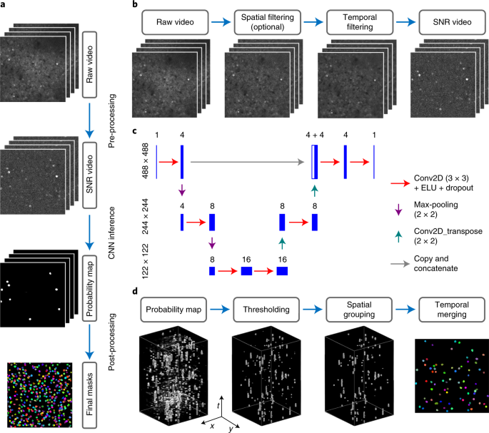
ABSTRACT Fluorescent genetically encoded calcium indicators and two-photon microscopy help understand brain function by generating large-scale in vivo recordings in multiple animal models.

Automatic, fast and accurate active neuron segmentation is critical when processing these videos. Here we developed and characterized a novel method, Shallow U-Net Neuron Segmentation

(SUNS), to quickly and accurately segment active neurons from two-photon fluorescence imaging videos. We used temporal filtering and whitening schemes to extract temporal features associated

with active neurons, and used a compact shallow U-Net to extract spatial features of neurons. Our method was both more accurate and an order of magnitude faster than state-of-the-art

techniques when processing multiple datasets acquired by independent experimental groups; the difference in accuracy was enlarged when processing datasets containing few manually marked

ground truths. We also developed an online version, potentially enabling real-time feedback neuroscience experiments. Access through your institution Buy or subscribe This is a preview of

subscription content, access via your institution ACCESS OPTIONS Access through your institution Access Nature and 54 other Nature Portfolio journals Get Nature+, our best-value

online-access subscription $29.99 / 30 days cancel any time Learn more Subscribe to this journal Receive 12 digital issues and online access to articles $119.00 per year only $9.92 per issue

Learn more Buy this article * Purchase on SpringerLink * Instant access to full article PDF Buy now Prices may be subject to local taxes which are calculated during checkout ADDITIONAL

ACCESS OPTIONS: * Log in * Learn about institutional subscriptions * Read our FAQs * Contact customer support SIMILAR CONTENT BEING VIEWED BY OTHERS ACCURATE NEURON SEGMENTATION METHOD FOR

ONE-PHOTON CALCIUM IMAGING VIDEOS COMBINING CONVOLUTIONAL NEURAL NETWORKS AND CLUSTERING Article Open access 09 August 2024 RAPID DETECTION OF NEURONS IN WIDEFIELD CALCIUM IMAGING DATASETS

AFTER TRAINING WITH SYNTHETIC DATA Article Open access 01 April 2023 A DEEP-LEARNING APPROACH FOR ONLINE CELL IDENTIFICATION AND TRACE EXTRACTION IN FUNCTIONAL TWO-PHOTON CALCIUM IMAGING

Article Open access 22 March 2022 DATA AVAILABILITY The trained network weights, and the optimal hyperparameters can be accessed at

https://github.com/YijunBao/SUNS_paper_reproduction/tree/main/paper_reproduction/training%20results. The output masks of all neuron segmentation algorithms can be accessed at

https://github.com/YijunBao/SUNS_paper_reproduction/tree/main/paper_reproduction/output%20masks%20all%20methods. We used three public datasets to evaluate the performance of SUNS and other

neuron segmentation algorithms. We used the videos of ABO dataset from https://github.com/AllenInstitute/AllenSDK/wiki/Use-the-Allen-Brain-Observatory-%E2%80%93-Visual-Coding-on-AWS, and we

used the corresponding manual labels created from our previous work, https://github.com/soltanianzadeh/STNeuroNet/tree/master/Markings/ABO. We used the Neurofinder dataset from

https://github.com/codeneuro/neurofinder, and we used the corresponding manual labels created from our previous work,

https://github.com/soltanianzadeh/STNeuroNet/tree/master/Markings/Neurofinder. We used the videos and manual labels of CaImAn dataset from https://zenodo.org/record/1659149. A more detailed

description of how we used these dataset can be found in the readme of https://github.com/YijunBao/SUNS_paper_reproduction/tree/main/paper_reproduction. CODE AVAILABILITY Code for SUNS can

be accessed at https://github.com/YijunBao/Shallow-UNet-Neuron-Segmentation_SUNS51. The version to reproduce the results in this paper can be accessed at

https://github.com/YijunBao/SUNS_paper_reproduction52. REFERENCES * Akerboom, J. et al. Genetically encoded calcium indicators for multi-color neural activity imaging and combination with

optogenetics. _Front. Mol. Neurosci._ 6, 2 (2013). Article  Google Scholar  * Chen, T.-W. et al. Ultrasensitive fluorescent proteins for imaging neuronal activity. _Nature_ 499, 295–300

(2013). Article  Google Scholar  * Dana, H. et al. High-performance calcium sensors for imaging activity in neuronal populations and microcompartments. _Nat. Methods_ 16, 649–657 (2019).

Article  Google Scholar  * Helmchen, F. & Denk, W. Deep tissue two-photon microscopy. _Nat. Methods_ 2, 932–940 (2005). Article  Google Scholar  * Stringer, C. et al. Spontaneous

behaviors drive multidimensional, brainwide activity. _Science_ 364, eaav7893 (2019). Article  Google Scholar  * Grewe, B. F. et al. High-speed in vivo calcium imaging reveals neuronal

network activity with near-millisecond precision. _Nat. Methods_ 7, 399–405 (2010). Article  Google Scholar  * Soltanian-Zadeh, S. et al. Fast and robust active neuron segmentation in

two-photon calcium imaging using spatiotemporal deep learning. _Proc. Natl Acad. Sci. USA_ 116, 8554–8563 (2019). Article  Google Scholar  * Pnevmatikakis, E. A. Analysis pipelines for

calcium imaging data. _Curr. Opin. Neurobiol._ 55, 15–21 (2019). Article  Google Scholar  * Klibisz, A. et al. in _Deep Learning in Medical Image Analysis and Multimodal Learning for

Clinical Decision Support_ (eds. Cardoso, J. et al.) 285–293 (Springer, 2017). * Gao, S. Automated neuron detection. _GitHub_

https://github.com/iamshang1/Projects/tree/master/Advanced_ML/Neuron_Detection (2016). * Shen, S. P. et al. Automatic cell segmentation by adaptive thresholding (ACSAT) for large-scale

calcium imaging datasets. _eNeuro_ 5, ENEURO.0056-18.2018 (2018). * Spaen, Q. et al. HNCcorr: a novel combinatorial approach for cell identification in calcium-imaging movies. _eNeuro_ 6,

ENEURO.0304-18.2019 (2019). * Kirschbaum, E., Bailoni, A. & Hamprecht, F. A. DISCo for the CIA: deep learning, instance segmentation, and correlations for calcium imaging analysis. In

_Medical Image Computing and Computer Assisted Intervention_, (eds. Martel, A. L. et al.) 151–162 (Springer, 2020) * Apthorpe, N. J. et al. Automatic neuron detection in calcium imaging data

using convolutional networks. _Adv. Neural Inf. Process Syst._ 29, 3278–3286 (2016). Google Scholar  * Mukamel, E. A., Nimmerjahn, A. & Schnitzer, M. J. Automated analysis of cellular

signals from large-scale calcium imaging data. _Neuron_ 63, 747–760 (2009). Article  Google Scholar  * Maruyama, R. et al. Detecting cells using non-negative matrix factorization on calcium

imaging data. _Neural Netw._ 55, 11–19 (2014). Article  Google Scholar  * Pnevmatikakis, EftychiosA. et al. Simultaneous denoising, deconvolution, and demixing of calcium imaging data.

_Neuron_ 89, 285–299 (2016). Article  Google Scholar  * Pachitariu, M. et al. Suite2p: beyond 10,000 neurons with standard two-photon microscopy. Preprint at _biorXiv_

https://doi.org/10.1101/061507 (2017). * Petersen, A., Simon, N. & Witten, D. SCALPEL: extracting neurons from calcium imaging data. _Ann. Appl. Stat._ 12, 2430–2456 (2018). Article 

MathSciNet  Google Scholar  * Giovannucci, A. et al. CaImAn an open source tool for scalable calcium imaging data analysis. _eLife_ 8, e38173 (2019). Article  Google Scholar  * Sitaram, R.

et al. Closed-loop brain training: the science of neurofeedback. _Nat. Rev. Neurosci._ 18, 86–100 (2017). Article  Google Scholar  * Kearney, M. G. et al. Discrete evaluative and premotor

circuits enable vocal learning in songbirds. _Neuron_ 104, 559–575.e6 (2019). Article  Google Scholar  * Carrillo-Reid, L. et al. Controlling visually guided behavior by holographic

recalling of cortical ensembles. _Cell_ 178, 447–457.e5 (2019). Article  Google Scholar  * Rickgauer, J. P., Deisseroth, K. & Tank, D. W. Simultaneous cellular-resolution optical

perturbation and imaging of place cell firing fields. _Nat. Neurosci._ 17, 1816–1824 (2014). Article  Google Scholar  * Packer, A. M., Russell, L. E., Dalgleish, H. W. P. & Häusser, M.

Simultaneous all-optical manipulation and recording of neural circuit activity with cellular resolution in vivo. _Nat. Methods_ 12, 140–146 (2015). Article  Google Scholar  * Zhang, Z. et

al. Closed-loop all-optical interrogation of neural circuits in vivo. _Nat. Methods_ 15, 1037–1040 (2018). Article  Google Scholar  * Giovannucci, A. et al. OnACID: online analysis of

calcium imaging data in real time. In _Advances in Neural Information Processing Systems_ (eds. Guyon, I. et al.) (Curran Associates, 2017). * Wilt, B. A., James, E. F. & Mark, J. S.

Photon shot noise limits on optical detection of neuronal spikes and estimation of spike timing. _Biophys. J._ 104, 51–62 (2013). Article  Google Scholar  * Jiang, R. & Crookes, D.

Shallow unorganized neural networks using smart neuron model for visual perception. _IEEE Access._ 7, 152701–152714 (2019). Article  Google Scholar  * Ba, J. & Caruana, R. Do deep nets

really need to be deep? _Adv. Neural Inf. Process. Syst_. (2014). * Lei, F., Liu, X., Dai, Q. & Ling, B. W.-K. Shallow convolutional neural network for image classification. _SN Appl.

Sci._ 2, 97 (2019). Article  Google Scholar  * Yu, S. et al. A shallow convolutional neural network for blind image sharpness assessment. _PLoS One_ 12, e0176632 (2017). Article  Google

Scholar  * Ronneberger, O., Fischer, P. & Brox, T. _U-Net: Convolutional Networks for Biomedical Image Segmentation_ (Springer, 2015). * _Code Neurofinder_ (CodeNeuro, 2019);

http://neurofinder.codeneuro.org/ * Arac, A. et al. DeepBehavior: a deep learning toolbox for automated analysis of animal and human behavior imaging data. _Front. Syst. Neurosci._ 13, 20

(2019). Article  Google Scholar  * Shen, D., Wu, G. & Suk, H.-I. Deep learning in medical image analysis. _Annu. Rev. Biomed. Eng._ 19, 221–248 (2017). Article  Google Scholar  * Zhou,

P. et al. Efficient and accurate extraction of in vivo calcium signals from microendoscopic video data. _eLife._ 7, e28728 (2018). Article  Google Scholar  * Meyer, F. Topographic distance

and watershed lines. _Signal Process._ 38, 113–125 (1994). Article  Google Scholar  * Pnevmatikakis, E. A. & Giovannucci, A. NoRMCorre: an online algorithm for piecewise rigid motion

correction of calcium imaging data. _J. Neurosci. Methods_ 291, 83–94 (2017). Article  Google Scholar  * Keemink, S. W. et al. FISSA: a neuropil decontamination toolbox for calcium imaging

signals. _Sci. Rep._ 8, 3493 (2018). Article  Google Scholar  * Mitani, A. & Komiyama, T. Real-time processing of two-photon calcium imaging data including lateral motion artifact

correction. _Front. Neuroinform._ 12, 98 (2018). Article  Google Scholar  * Frankle, J. & Carbin, M. The lottery ticket hypothesis: finding sparse, trainable neural networks. In

_International Conference on Learning Representations_ (ICLR, 2019). * Yang, W. & Lihong, X. Lightweight compressed depth neural network for tomato disease diagnosis. _Proc. SPIE_

(2020). * Oppenheim, A., Schafer, R. & Stockham, T. Nonlinear filtering of multiplied and convolved signals. _IEEE Trans. Audio Electroacoust._ 16, 437–466 (1968). Article  Google

Scholar  * Szymanska, A. F. et al. Accurate detection of low signal-to-noise ratio neuronal calcium transient waves using a matched filter. _J. Neurosci. Methods_ 259, 1–12 (2016). Article 

Google Scholar  * Milletari, F., Navab, N. & Ahmadi, S. V-Net: fully convolutional neural networks for volumetric medical image segmentation. In _2016 Fourth International Conference on

3D Vision_ 565–571 (3DV, 2016). * Lin, T.-Y. et al. Focal loss for dense object detection. In _Proc. IEEE International Conference on Computer Vision_ 2980–2988 (IEEE, 2017). * de Vries, S.

E. J. et al. A large-scale standardized physiological survey reveals functional organization of the mouse visual cortex. _Nat. Neurosci._ 23, 138–151 (2020). Article  Google Scholar  *

Gilman, J. P., Medalla, M. & Luebke, J. I. Area-specific features of pyramidal neurons—a comparative study in mouse and rhesus monkey. _Cerebral Cortex._ 27, 2078–2094 (2016). Google

Scholar  * Ballesteros-Yáñez, I. et al. Alterations of cortical pyramidal neurons in mice lacking high-affinity nicotinic receptors. _Proc. Natl Acad. Sci. USA_ 107, 11567–11572 (2010).

Article  Google Scholar  * Bao, Y. YijunBao/Shallow-UNet-Neuron-Segmentation_SUNS. _Zenodo_ https://doi.org/10.5281/zenodo.4638171 (2021). * Bao, Y. YijunBao/SUNS_paper_reproduction.

_Zenodo_ https://doi.org/10.5281/zenodo.4638135 (2021). Download references ACKNOWLEDGEMENTS We acknowledge support from the BRAIN Initiative (NIH 1UF1-NS107678, NSF 3332147), the NIH New

Innovator Program (1DP2-NS111505), the Beckman Young Investigator Program, the Sloan Fellowship and the Vallee Young Investigator Program received by Y.G. We acknowledge Z. Zhu for early

characterization of the SUNS. AUTHOR INFORMATION AUTHORS AND AFFILIATIONS * Department of Biomedical Engineering, Duke University, Durham, NC, USA Yijun Bao, Somayyeh Soltanian-Zadeh, Sina

Farsiu & Yiyang Gong * Department of Ophthalmology, Duke University Medical Center, Durham, NC, USA Sina Farsiu * Department of Neurobiology, Duke University, Durham, NC, USA Yiyang Gong

Authors * Yijun Bao View author publications You can also search for this author inPubMed Google Scholar * Somayyeh Soltanian-Zadeh View author publications You can also search for this

author inPubMed Google Scholar * Sina Farsiu View author publications You can also search for this author inPubMed Google Scholar * Yiyang Gong View author publications You can also search

for this author inPubMed Google Scholar CONTRIBUTIONS Y.G. conceived and designed the project. Y.B. and Y.G. implemented the code for SUNS. Y.B. and S.S.-Z. implemented the code for other

algorithms for comparison. Y.B. ran the experiment. Y.B., S.S.-Z., S.F. and Y.G. analysed the data. Y.B., S.S.-Z., S.F. and Y.G. wrote the paper. CORRESPONDING AUTHORS Correspondence to

Yijun Bao or Yiyang Gong. ETHICS DECLARATIONS COMPETING INTERESTS The authors declare no competing interests. ADDITIONAL INFORMATION PEER REVIEW INFORMATION _Nature Machine Intelligence_

thanks Xue Han and the other, anonymous, reviewer(s) for their contribution to the peer review of this work. PUBLISHER’S NOTE Springer Nature remains neutral with regard to jurisdictional

claims in published maps and institutional affiliations. EXTENDED DATA EXTENDED DATA FIG. 1 THE AVERAGE CALCIUM RESPONSE FORMED THE TEMPORAL FILTER KERNEL. We determined the temporal matched

filter kernel by averaging calcium transients within a moderate SNR range; these transients likely represent the temporal response to single action potentials2. A, Example data show all

background-subtracted fluorescence calcium transients of all GT neurons in all videos in the ABO 275 μm dataset that showed peak SNR (pSNR) in the regime 6 < pSNR < 8 (_gray_). We

minimized crosstalk from neighboring neurons by excluding transients during time periods when neighboring neurons also had transients. We normalized all transients such that their peak

values were unity, and then averaged these normalized transients into an averaged spike trace (_red_). We used the portion of the average spike trace above e–1 (_blue dashed line_) as the

final template kernel. B, When analyzing performance on the ABO 275 μm dataset through ten-fold leave-one-out cross-validation, using the temporal kernel determined in (A) within our

temporal filter scheme achieved significantly higher _F_1 score than not using a temporal filter or using an unmatched filter (*_P_ < 0.05, **_P_ < 0.005; two-sided Wilcoxon

signed-rank test, _n_ = 10 videos) and achieved a slightly higher _F_1 score than using a single exponentially decaying kernel (_P_ = 0.77; two-sided Wilcoxon signed-rank test, _n_ = 10

videos). Error bars are s.d. The gray dots represent scores for the test data for each round of cross-validation. The unmatched filter was a moving-average filter over 60 frames. C-D, are

analogous to (A-B), but for the Neurofinder dataset. We determined the filter kernel using videos 04.01 and 04.01.test. EXTENDED DATA FIG. 2 THE COMPLEXITY OF THE CNN ARCHITECTURE CONTROLLED

THE TRADEOFF BETWEEN SPEED AND ACCURACY. We explored multiple potential CNN architectures to optimize performance. A-D, Various CNN architectures having depths of (A) two, (B) three, (C)

four, or (D) five. For the three-depth architecture, we also tested different numbers of skip connections, ReLU (Rectified Linear Unit) instead of ELU (Exponential Linear Unit) as the

activation function, and separable Conv2D instead of Conv2D in the encoding path. The dense five-depth model mimicked the model used in UNet2Ds9. The legend ‘0/_n__i_ + _n__i_’ represents

whether the skip connection was used (_n__i_ + _n__i_) or not used (0 + _n__i_). E, The _F_1 score and processing speed of SUNS using various CNN architectures when analyzing the ABO 275 μm

dataset through ten-fold leave-one-out cross-validation. The right panel zooms in on the rectangular region in the left panel. Error bars are s.d. The legend (_n_1, _n_2, …, _n__k_)

describes architectures with _k_-depth and _n__i_ channels at the _i_th depth. We determined that the three-depth model, (4,8,16), using one skip connection at the shallowest layer, ELU, and

full Conv2D (Fig. 1c), had a good trade-off between speed and accuracy; we used this architecture as the SUNS architecture throughout the paper. One important drawback of the ReLU

activation function was its occasional (20% of the time) failure during training, compared to negligible failure levels for the ELU activation function. EXTENDED DATA FIG. 3 THE _F_1 SCORE

OF SUNS WAS ROBUST TO MODERATE VARIATION OF TRAINING AND POST-PROCESSING PARAMETERS. We tested if the accuracy of SUNS when analyzing the ABO 275 μm dataset within the ten-fold leave-one-out

cross-validation relied on intricate tuning of the algorithm’s hyperparameters. The evaluated training parameters included (A) the threshold of the SNR video (_th_SNR) and (B) the training

batch size. The evaluated post-processing parameters included (C) the threshold of probability map (_th_prob), (D) the minimum neuron area (_th_area), (E) the threshold of COM distance

(_th_COM), and (F) the minimum number of consecutive frames (_th_frame). The solid blue lines are the average _F_1 scores, and the shaded regions are mean ± one s.d. When evaluating the

post-processing parameters in (C-F), we fixed each parameter under investigation at the given values and simultaneously optimized the _F_1 score over the other parameters. Variations in

these hyperparameters produced only small variations in the _F_1 performance. The orange lines show the _F_1 score (_solid_) ± one s.d. (_dashed_) when we optimized all four post-processing

parameters simultaneously. The similarity between the _F_1 scores on the blue lines and the scores on the orange lines suggest that optimizing for three or four parameters simultaneously

achieved similar optimized performance. Moreover, the relatively consistent _F_1 scores on the blue lines suggest that our algorithm did not rely on intricate hyperparameter tuning. EXTENDED

DATA FIG. 4 THE PERFORMANCE OF SUNS WAS BETTER THAN THAT OF OTHER METHODS IN THE PRESENCE OF INTENSITY NOISE OR MOTION ARTIFACTS. The (A, D) recall, (B, E) precision, and (C, F) _F_1 score

of all the (A-C) batch and (D-F) online segmentation algorithms in the presence of increasing intensity noise. The test dataset was the ABO 275 μm data with added random noise. The relative

noise strength was represented by the ratio of the standard deviation of the random noise amplitude to the mean fluorescence intensity. As expected, the _F_1 scores of all methods decreased

as the noise amplitude grew. The _F_1 of SUNS was greater than the _F_1’s of all other methods at all noise intensities. G-L, are in the same format of (A-F), but show the performance with

the presence of increasing motion artifacts. The motion artifacts strength was represented by the standard deviation of the random movement amplitude (unit: pixels). As expected, the _F_1

scores of all methods decreased as the motion artifacts became stronger. The _F_1 of SUNS was greater than the _F_1’s of all other methods at all motion amplitudes. STNeuroNet and CaImAn

batch were the most sensitive to strong motion artifacts, likely because they rely on accurate 3D spatiotemporal structures of the video. On the contrary, SUNS relied more on the 2D spatial

structure, so it retained the accuracy better when spatial structures changed position over different frames. EXTENDED DATA FIG. 5 SUNS ACCURATELY MAPPED THE SPATIAL EXTENT OF EACH NEURON

EVEN IF THE SPATIAL FOOTPRINTS OF NEIGHBORING CELLS OVERLAPPED. SUNS segmented active neurons within each individual frame, and then accurately collected and merged the instances belonging

to the same neurons. We selected two example pairs of overlapping neurons from the ABO video 539670003 identified by SUNS, and showed their traces and instances when they were activated

independently. A, The SNR images of the region surrounding the selected neurons. The left image is the maximum projection of the SNR video over the entire recording time, which shows the two

neurons were active and overlapping. The right images are single-frame SNR images at two different time points, each at the peak of a fluorescence transient where only one of the two

neurons was active. The segmentation of each neuron generated by SUNS is shown as a contour with a different color. The scale bar is 3 μm. B, The temporal SNR traces of the selected neurons,

matched to the colors of their contours in (A). Because the pairs of neurons overlapped, their fluorescence traces displayed substantial crosstalk. The dash markers above each trace show

the active periods of each neuron determined by SUNS. The colored triangles below each trace indicate the manually-selected time of the single-frame images shown in (A). C-D, are parallel to

(A-B), but for a different overlapping neuron pair. E, We quantified the ability to find overlapped neurons for each segmentation algorithm using the recall score. We divided the ground

truth neurons in all the ABO videos into two groups: neurons without and with overlap with other neurons. We then computed the recall scores for both groups. The recall of SUNS on spatially

overlapping neurons was not significantly lower (and was numerically higher) than the recall of SUNS on non-spatially overlapping neurons (_P_ > 0.8, one-sided Wilcoxon rank-sum test, _n_

 = 10 videos; n.s.l. – not significantly lower). Therefore, the performance of SUNS on overlapped neurons was at least equally good as the performance of SUNS on non-overlapped neurons.

Moreover, the recall scores of SUNS in both groups were comparable to or significantly higher than that of other methods in those groups (**_P_ < 0.005, n.s. – not significant; two-sided

Wilcoxon signed-rank test, _n_ = 10 videos; error bars are s.d.). The gray dots represent the scores on the test data for each round of cross-validation. EXTENDED DATA FIG. 6 EACH

PRE-PROCESSING STEP AND THE CNN CONTRIBUTED TO THE ACCURACY OF SUNS AT THE COST OF LOWER SPEED. We evaluated the contribution of each pre-processing option (spatial filtering, temporal

filtering, and SNR normalization) and the CNN option to SUNS. The reference algorithm (SUNS) used all options except spatial filtering. We compared the performance of this reference

algorithm to the performance with additional spatial filtering (optional SF), without temporal filtering (no TF), without SNR normalization (no SNR), and without the CNN (no CNN) when

analyzing the ABO 275 μm dataset through ten-fold leave-one-out cross-validation. A, The recall, precision, and _F_1 score of these variants. The temporal filtering, SNR normalization, and

CNN each significantly contributed to the overall accuracy, but the impact of spatial filtering was not significant (*_P_ < 0.05, **_P_ < 0.005, n.s. - not significant; two-sided

Wilcoxon signed-rank test, _n_ = 10 videos; error bars are s.d.). The gray dots represent the scores on the test data for each round of cross-validation. B, The speed and _F_1 score of these

variants. Eliminating temporal filtering or the CNN significantly increased the speed, while adding spatial filtering or eliminating SNR normalization significantly lowered the speed (**_P_

 < 0.005; two-sided Wilcoxon signed-rank test, _n_ = 10 videos; error bars are s.d.). The light color dots represent _F_1 scores and speeds for the test data for each round of

cross-validation. The execution of SNR normalization was fast (~0.07 ms/frame). However, eliminating SNR normalization led to a much lower optimal _th_prob, and thus increased the number of

active pixels and decreased precision. In addition, ‘no SNR’ had lower speed than the complete SUNS algorithm due to the increased post-processing computation workload for managing the

additional active pixels and regions. EXTENDED DATA FIG. 7 THE RECALL, PRECISION, AND _F_1 SCORE OF SUNS WERE SUPERIOR TO THAT OF OTHER METHODS ON A VARIETY OF DATASETS. A, Training on one

ABO 275 μm video and testing on nine ABO 275 μm videos (each data point is the average over each set of nine test videos, _n_ = 10); B, Training on ten ABO 275 μm videos and testing on ten

ABO 175 μm videos (_n_ = 10); C, Training on one Neurofinder video and testing on one paired Neurofinder video (_n_ = 12); D, Training on three-quarters of one CaImAn video and testing on

the remaining quarter of the same CaImAn video (_n_ = 16). The _F_1 scores of SUNS were mostly significantly higher than the _F_1 scores of other methods (*_P_ < 0.05, **_P_ < 0.005,

***_P_ < 0.001, n.s. - not significant; two-sided Wilcoxon signed-rank test; error bars are s.d.). The gray dots represent the individual scores for each round of cross-validation.

EXTENDED DATA FIG. 8 SUNS ONLINE OUTPERFORMED CAIMAN ONLINE IN ACCURACY AND SPEED WHEN PROCESSING A VARIETY OF DATASETS. A,E, Training on one ABO 275 μm video and testing on nine ABO 275 μm

videos (each data point is the average over each set of nine test videos, _n_ = 10); B, F, Training on ten ABO 275 μm videos and testing on ten ABO 175 μm videos (_n_ = 10); C, G, Training

on one Neurofinder video and testing on one paired Neurofinder video (_n_ = 12); D, H, Training on three-quarters of one CaImAn video and testing on the remaining quarter of the same CaImAn

video (_n_ = 16). The _F_1 score and processing speed of SUNS online were significantly higher than the _F_1 score and speed of CaImAn Online (**_P_ < 0.005, ***_P_ < 0.001; two-sided

Wilcoxon signed-rank test; error bars are s.d.). The gray dots in (A-D) represent individual scores for each round of cross-validation. The light color dots in (E-G) represent _F_1 scores

and speeds for the test data for each round of cross-validation. The light color markers in (H) represent _F_1 scores and speeds for the test data for each round of cross-validation

performed on different CaImAn videos. We updated the baseline and noise regularly after initialization for the Neurofinder dataset, but did not do so for other datasets. EXTENDED DATA FIG. 9

CHANGING THE FREQUENCY OF UPDATING THE NEURON MASKS MODULATED TRADE-OFFS BETWEEN SUNS ONLINE’S RESPONSE TIME TO NEW NEURONS AND SUNS ONLINE’S PERFORMANCE METRICS. The (A-C) _F_1 score and

(D-F) speed of SUNS online increased as the number of frames per update (_n_merge) increased for the (A, D) ABO 275 μm, (B, E) Neurofinder, and (C, F) CaImAn datasets. The solid line is the

average, and the shading is one s.d. from the average (_n_ = 10, 12, and 16 cross-validation iterations for the three datasets). In (A-C), the green lines show the _F_1 score (_solid_) ± one

s.d. (_dashed_) of SUNS batch. The _F_1 score and speed generally increased as _n_merge increased. For example, the _F_1 score and speed when using _n_merge = 500 were respectively higher

than the _F_1 score and speed when using _n_merge = 20, and some of the differences were significant (*_P_ < 0.05, **_P_ < 0.005, ***_P_ < 0.001, n.s. - not significant; two-sided

Wilcoxon signed-rank test; _n_ = 10, 12, and 16, respectively). We updated the baseline and noise regularly after initialization for the Neurofinder dataset, but did not do so for other

datasets. The _n_merge was inversely proportional to the update frequency or the responsiveness of SUNS online to the appearance of new neurons. A trade-off exists between this

responsiveness and the accuracy and speed of SUNS online. At the cost of less responsiveness, a higher _n_merge allowed the accumulation of temporal information and improved the accuracy of

neuron segmentations. Likewise, a higher _n_merge improved the speed because it reduced the occurrence of computations for aggregating neurons. EXTENDED DATA FIG. 10 UPDATING THE BASELINE

AND NOISE AFTER INITIALIZATION INCREASED THE ACCURACY OF SUNS ONLINE AT THE COST OF LOWER SPEED. We compared the _F_1 score and speed of SUNS online with or without baseline and noise update

for the (A) ABO 275 μm, (B) Neurofinder, and (C) CaImAn datasets. The _F_1 scores with baseline and noise update were generally higher, but the speeds were slower (*_P_ < 0.05, **_P_ 

< 0.005, ***_P_ < 0.001, n.s. - not significant; two-sided Wilcoxon signed-rank test; error bars are s.d.). The light color dots represent _F_1 scores and speeds for the test data for

each round of cross-validation. The improvement in the _F_1 score was larger as the baseline fluctuation becomes more significant. D, Example processing time per frame of SUNS online with

baseline and noise update on Neurofinder video 02.00. The lower inset zooms in on the data from the red box. The upper inset is the distribution of processing time per frame. The processing

time per frame was consistently faster than the microscope recording rate (125 ms/frame). The first few frames after initialization were faster than the following frames, because the

baseline and noise update was not performed in these frames. SUPPLEMENTARY INFORMATION SUPPLEMENTARY INFORMATION Supplementary Figs. 1–14, Tables 1–10 and Methods. REPORTING SUMMARY

SUPPLEMENTARY VIDEO 1 Demonstration of how SUNS online gradually found new neurons on an example raw video. The example video is selected frames in the fourth quadrant of the video YST from

the CaImAn dataset. We showed the results of the SUNS online without the ‘tracking’ option enabled (left) and with the ‘tracking’ option enabled (right). The red contours were the segmented

neurons from all frames before the current frame. We updated the identified neuron contours every second (ten frames), so the red neuron contours appeared with some delay after the neurons’

initial activation. The green contours in the right panels were the neurons found in previous frames and appeared as active in the current frames. Such tracked activity enables follow-up

analysis of animal behaviours or brain network structures in real-time feedback neuroscience experiments. SUPPLEMENTARY VIDEO 2 Demonstration of how SUNS online gradually found new neurons

on an example SNR video. The example video is selected frames in the fourth quadrant of the video YST from the CaImAn dataset after pre-processing and conversion to an SNR video. We showed

the results of the SUNS online without the ‘tracking’ option enabled (left) and with the ‘tracking’ option enabled (right). The red contours were the segmented neurons from all frames before

the current frame. We updated the identified neuron contours every second (ten frames), so the red neuron contours appeared with some delay after the neurons’ initial activation. The green

contours in the right panels were the neurons found in previous frames and appeared as active in the current frames. Such tracked activity enables follow-up analysis of animal behaviours or

brain network structures in real-time feedback neuroscience experiments. RIGHTS AND PERMISSIONS Reprints and permissions ABOUT THIS ARTICLE CITE THIS ARTICLE Bao, Y., Soltanian-Zadeh, S.,

Farsiu, S. _et al._ Segmentation of neurons from fluorescence calcium recordings beyond real time. _Nat Mach Intell_ 3, 590–600 (2021). https://doi.org/10.1038/s42256-021-00342-x Download

citation * Received: 19 October 2020 * Accepted: 09 April 2021 * Published: 20 May 2021 * Issue Date: July 2021 * DOI: https://doi.org/10.1038/s42256-021-00342-x SHARE THIS ARTICLE Anyone

you share the following link with will be able to read this content: Get shareable link Sorry, a shareable link is not currently available for this article. Copy to clipboard Provided by the

Springer Nature SharedIt content-sharing initiative