Reader TTS

ABSTRACT Timescales characterize the pace of change for many dynamic processes in nature. They are usually estimated by fitting the exponential decay of data autocorrelation in the time or

frequency domain. Here we show that this standard procedure often fails to recover the correct timescales due to a statistical bias arising from the finite sample size. We develop an

alternative approach to estimate timescales by fitting the sample autocorrelation or power spectrum with a generative model based on a mixture of Ornstein–Uhlenbeck processes using adaptive

approximate Bayesian computations. Our method accounts for finite sample size and noise in data and returns a posterior distribution of timescales that quantifies the estimation uncertainty

and can be used for model selection. We demonstrate the accuracy of our method on synthetic data and illustrate its application to recordings from the primate cortex. We provide a

customizable Python package that implements our framework via different generative models suitable for diverse applications. SIMILAR CONTENT BEING VIEWED BY OTHERS THE BRAIN TIME TOOLBOX, A

SOFTWARE LIBRARY TO RETUNE ELECTROPHYSIOLOGY DATA TO BRAIN DYNAMICS Article 20 June 2022 PARAMETERIZING NEURAL POWER SPECTRA INTO PERIODIC AND APERIODIC COMPONENTS Article 23 November 2020

THE SIGNIFICANCE OF NEURAL INTER-FREQUENCY POWER CORRELATIONS Article Open access 30 November 2021 MAIN Dynamic changes in many stochastic processes occur over typical periods known as

timescales. Accurate measurements of timescales from experimental data are necessary to uncover the mechanisms controlling the dynamics of underlying processes and reveal their

function1,2,3,4,5. The timescales of a stochastic process are defined by the exponential decay rates of its autocorrelation function. Accordingly, timescales are usually estimated by fitting

the autocorrelation of a sample time-series with exponential decay functions1,5,6,7,8,9,10,11,12,13,14,15, or fitting the shape of the sample power spectral density (PSD) with a Lorentzian

function3,16. However, the sample autocorrelation values computed from a finite time-series systematically deviate from the true autocorrelation17,18,19,20,21,22. This bias is exacerbated by

the lack of independence between the samples, especially when the timescales are large and the time-series is short23,24,25. The magnitude of bias generally depends on the length of the

sample time-series, but also on the value of the true autocorrelation at each time-lag. The expected value and variance of the autocorrelation bias can be derived analytically in simple

cases (for example, the single-timescale Markov process)17,20, but become intractable for more general processes with multiple timescales or an additional temporal structure. Moreover, as

the bias depends on the true autocorrelation itself, which is unknown, it cannot be easily corrected. The statistical bias deforms the shape of empirical autocorrelations and—according to

the Wiener–Khinchin theorem26—PSDs; it can therefore affect the timescales estimated by direct fitting methods. Fitting the sample autocorrelation of an Ornstein–Uhlenbeck (OU) process with

an exponential decay function results in systematic errors in the estimated timescale and confidence interval27. It is possible to fit the time-series directly with an autoregressive model

to avoid these errors, without using autocorrelation or PSD27,28. However, the advantage of autocorrelation is that factors unrelated to the dynamics of the processes under study (for

example, slow activity drifts) can be efficiently removed with resampling methods29,30,31,32. By contrast, accounting for irrelevant factors in the autoregressive model requires the addition

of components that must all be fitted to the data. Fitting the summary statistic such as autocorrelation or PSD is therefore attractive, but how the statistical bias affects the estimated

timescales was not studied systematically. We show that large systematic errors in estimated timescales arise from the statistical bias due to a finite sample size. To correct for the bias,

we develop a flexible computational framework based on adaptive approximate Bayesian computations (aABCs) that estimate timescales by fitting the autocorrelation or PSD with a generative

model. The aABC algorithm approximates the multivariate posterior distribution of parameters of a generative model using population Monte Carlo sampling33. The posterior distributions can be

used for quantifying the estimation uncertainty and model selection. Our computational framework can be adapted to various types of data and can find broad applications in neuroscience,

physics and other fields. RESULTS BIAS IN TIMESCALES ESTIMATED BY DIRECT FITTING Timescales of a stochastic process \(A(t^{\prime} )\) are defined by the exponential decay rates of its

autocorrelation function, that is, the correlation between values of the process at time points separated by a time lag _t_. For stationary processes, the autocorrelation function only

depends on _t_: $${\mathrm{AC}}(t)=\frac{{{{\rm{E}}}}{\left[\left(A(t^{\prime} )-\mu \right)\left(A(t^{\prime} +t)-\mu \right)\right]}_{t^{\prime} }}{{\sigma }^{2}}.$$ (1) Here _μ_ and _σ_2

are the mean and variance of the process, respectively, and \({{{\rm{E}}}}{[\cdot ]}_{t^{\prime} }\) is the expectation over \(t^{\prime}\). For empirical data, the true values of _μ_ and

_σ_ are unknown. Hence, several estimators of the sample autocorrelation were proposed that use different estimators for the sample mean \(\hat{\mu }\) and sample variance \({\hat{\sigma

}}^{2}\) (see the “Computing sample autocorrelation” section in the Methods)17,18. The sample autocorrelation can also be computed as the inverse Fourier transform of the PSD on the basis of

the Wiener–Khinchin theorem26. However, for any of these methods, the sample autocorrelation is a biased estimator: the sample autocorrelation values for a finite-length time-series

systematically deviate from the ground-truth autocorrelation17,18,19,20,21,22 (Fig. 1 and Supplementary Fig. 1). This statistical bias deforms the shape of the sample autocorrelation or PSD

and may affect the estimation of timescales by direct fitting of the shape. To investigate the impact of autocorrelation bias on the timescales estimated by direct exponential fitting, we

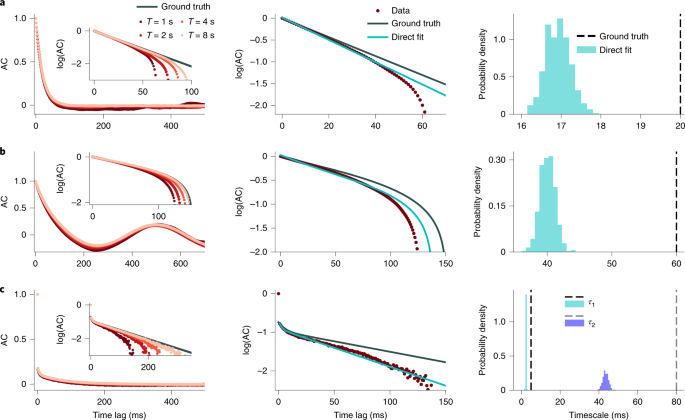
tested how accurately this procedure recovers the correct timescales on synthetic data for which the ground truth is known. We generated synthetic data from several stochastic processes for

which the autocorrelation function can be computed analytically (see the “Generative models” section in the Methods). The exponential decay rates of the analytical autocorrelation provide

the ground-truth timescales. We considered three ground-truth processes that differed by the number of timescales, an additional temporal structure, and noise: (1) an OU process (Fig. 1a);

(2) a linear mixture of an OU process and oscillatory component (Fig. 1b, resembling the firing rate of a neuron modulated by a slow oscillation34,35); and (3) an inhomogeneous Poisson

process (often used to model spiking activity of neurons36) with the instantaneous rate modeled as a linear mixture of two OU processes with different timescales (Fig. 1c). For all three

processes, the sample autocorrelation exhibits a negative bias, that is, the values of the sample autocorrelation are systematically below the ground-truth autocorrelation function (Fig. 1,

left). This bias is clearly visible in the logarithmic-linear scale, in which the ground-truth exponential decay turns into a straight line. The sample autocorrelation deviates from the

straight line and even becomes systematically negative at intermediate lags (and hence is not visible on the logarithmic scale) for processes with a strictly positive ground-truth

autocorrelation (Fig. 1a,c). The deviations from the ground truth are larger when the timescales are longer or when multiple timescales are involved. The negative bias decreases for longer

trial durations (Fig. 1, left inset) but it is still substantial for realistic trial durations such as in neuroscience data. Due to the negative bias, a direct fit of the sample

autocorrelation with the correct analytical function cannot recover the ground-truth timescales (Fig. 1, middle, right; Supplementary Figs. 2 and 3). When increasing the duration of each

trial, the timescales obtained from the direct fits bcome more closely aligned with the ground-truth values (Supplementary Fig. 4). This observation indicates that timescales estimated from

datasets with different trial durations cannot be directly compared, as differences in the estimation bias may result in misleading interpretations. Direct fitting of a sample

autocorrelation—even with a known correct analytical form—is therefore not a reliable method for measuring timescales in experimental data. Bias-correction methods based on parametric

bootstrapping can mitigate the estimation bias of timescales from direct fits37. However, as the amount of bias depends on the ground-truth timescales, such corrections cannot guarantee

accurate estimates in all cases (Supplementary Fig. 5). Alternatively, we can estimate timescales in the frequency domain by fitting the PSD shape with a Lorentzian function, equation (5),

which is the ground-truth PSD for a stochastic process with an exponentially decaying autocorrelation3,16. Comparison of the ground-truth PSD with the sample PSD of an OU process with finite

duration reveals that the statistical bias also persists in the frequency domain (Supplementary Fig. 6a). Due to this bias, the estimated timescale deviates from the ground truth by the

amount that depends on the fitted frequency range. Although careful choice of the fitted frequency range can improve the estimation accuracy (Supplementary Fig. 6b), without knowing the

ground-truth timescale, there is no principled way to choose the correct range for all cases. Slightly changing the fitted frequency range can produce large errors in estimated timescale,

especially in the presence of additional noise, for example, spiking activity. ESTIMATING TIMESCALES BY FITTING GENERATIVE MODELS WITH AABC As direct fitting methods cannot estimate

timescales reliably, we developed an alternative computational framework based on fitting the sample autocorrelation (or PSD) with a generative model. Using a model with known ground-truth

timescales, we can generate synthetic data that match the essential statistics of the observed data, that is, with the same duration and number of trials, mean and variance. Hence the sample

autocorrelations (or PSDs) of the synthetic and observed data will be affected by a similar statistical bias when their shapes match. We chose a linear mixture of OU processes (one for each

estimated timescale) as a generative model, which, if necessary, could be augmented with an additional temporal structure (such as oscillations) and noise. The advantage of using a mixture

of OU processes is that the analytical autocorrelation function of this mixture explicitly defines the timescales. We set the number of components in the generative model according to our

hypothesis on the autocorrelation in the data, for example, the number of timescales, additional temporal structure and noise (see the “Generative models” section in the Methods). We then

optimize parameters of the generative model to match the shape of the autocorrelation (or PSD) between the synthetic and observed data. The timescales of the optimized generative model

provide an unbiased estimation of timescales in the data. Calculating the likelihood for complex generative models can be computationally expensive or even intractable. We therefore optimize

the generative model parameters using aABC (Fig. 2)33, an iterative algorithm that minimizes the distance between the summary statistic of synthetic and observed data (Fig. 2 and the

“Optimizing generative model parameters with aABC” section in the Methods). Depending on the application, we can choose a summary statistic in the time (autocorrelation) or frequency (PSD)

domains. On each iteration, we draw a set of parameters of the generative model, either from a prior distribution (first iteration) or a proposal distribution, and generate synthetic data

using these parameter samples. The sampled parameters are accepted if the distance _d_ between the summary statistic of the observed and synthetic data is smaller than a selected error

threshold _ε_. The last set of accepted parameter samples provides an approximation of the posterior distribution. The joint posterior distribution quantifies the estimation uncertainty

taking into account the stochasticity of the observed data (Supplementary Fig. 7). We implemented this algorithm in the abcTau Python package including different types of summary statistics

and generative models (see the “abcTau Python package” in the Methods). We marginalize the multivariate posterior distribution over all other parameters of the generative model to visualize

the posterior distribution of a parameter (such as a timescale). We illustrate our method on synthetic data from the processes described in the previous section, using the autocorrelation as

the summary statistic (compare Fig. 3 with Fig. 1). For all three processes, the shape of the sample autocorrelation of the observed data is accurately reproduced by the autocorrelation of

synthetic data generated using the maximum a posteriori (MAP) estimate of parameters from the joint multivariate posterior distribution (Fig. 3, left). The posterior distributions inferred

by aABC include the ground-truth timescales (Fig. 3, middle). The posterior variance quantifies the estimation uncertainty. In our simulations, the number of trials controls the

signal-to-noise ratio in sample autocorrelation and consequently the width of the posteriors (Supplementary Fig. 8). The aABC method also recovers the ground-truth timescales by fitting the

sample PSD without tuning the frequency range, even in the presence of multiple timescales, additional spiking noise (Supplementary Fig. 9) or multiple oscillatory components (Supplementary

Fig. 10). Moreover, the aABC method can uncover slow oscillations in signals that do not exhibit clear peaks in PSD due to the short duration of the time-series and the low frequency

resolution (Supplementary Fig. 9c). The aABC method can be used in combination with any method for computing the PSD (for example, any window functions for removing the spectral leakage), as

the exact same method applied to synthetic data would alter their sample PSD in the same way. Different summary statistics and fitting ranges may be preferred depending on the application.

For example, autocorrelations allow for using additional correction methods such as jittering31, whereas PSD estimation can be improved with filtering or multitapers38. Furthermore,

selecting a smaller maximum time-lag when fitting autocorrelations prevents overfitting to noise in the autocorrelation tail. The choice of summary statistic (metric and fitting range) can

influence the shape of the approximated posterior (for example, posterior width), but the posteriors peak close to the ground-truth timescales as long as the same summary statistic is used

for observed and synthetic data (Supplementary Fig. 11). The advantage of such behavior is particularly visible when changing the range over which we compute the summary statistics (for

example, minimum and maximum frequency in PSD), which affects direct fit but not aABC estimates (Supplementary Fig. 6). In the aABC algorithm we set a multivariate uniform prior distribution

over the parameters of the generative model. The ranges of uniform prior should be broad enough to include the ground-truth values. Selecting broader priors does not affect the shape of

posteriors and only slows down the fitting procedure (Supplementary Fig. 12). Hence we can set wide prior distributions when a reasonable range of parameters is unknown. Timescales estimated

from the direct exponential fits can be used as a potential lower bound for the priors. We evaluated the reliability of the aABC method on a wide range of timescales and trial durations and

compared the results to direct fitting (Supplementary Fig. 13). The estimation error of direct fitting increases when trial durations become short relative to the timescale, whereas the

aABC method always returns reliable estimates. However, the estimation of the full posterior comes at a price of higher computational costs (Supplementary Table 3) than point estimates;

thus, the direct fit of the sample autocorrelation may be preferred when the long time-series data are available so that statistical bias does not corrupt the results. To empirically verify

whether this is the case, we implemented a pre-processing algorithm in our Python package that uses parametric bootstrapping to return an approximate error bound of the direct fit estimates

(see Supplementary Fig. 14 and the “Pre-processing for evaluating quality of direct” section in the Methods). Fitting generative models with the aABC method provides a principled framework

for estimating timescales that can be used with different metrics in time or frequency domain. Furthermore, joint posterior distribution of the inferred parameters allows us to examine

correlations between different parameters, find manifolds of possible solutions, and identify a potential degeneracy in the parameter space (Supplementary Fig. 15). ESTIMATING THE TIMESCALE

OF ACTIVITY IN A BRANCHING NETWORK So far we have demonstrated that our aABC method accurately recovers the ground-truth timescales when the generative model and the process that produced

the observed data are the same. However, the inference of timescales using OU processes is broadly applicable when the mechanism that generated the exponential decay of autocorrelation in

the data is not an OU process. As an example, we tested our method on discrete-time data from an integer-valued autoregressive model with a known ground-truth autocorrelation function.

Specifically, we applied our method to estimate the timescale of the global activity in a branching network model, which is often used to study the operating regime of dynamics in neuronal

networks (Fig. 4a)39,40,41. We simulated the network model to generate the time-series data of the global activity. We then used aABC to fit the sample autocorrelation of these data with a

one-timescale OU process as a generative model. The inferred posterior is centered on the theoretically predicted timescale of the branching network, and the MAP estimate parameter

accurately reproduces the shape of the sample autocorrelation of the network activity (Fig. 4b,c). These results show that our framework can be used to estimate timescales in diverse types

of data. MODEL SELECTION WITH ABC The correct generative model (for example, the number of timescales) is usually unknown for experimental data. We thus need a procedure to select between

alternative hypotheses. Assuming that the autocorrelation or PSD is a sufficient summary statistic for estimating timescales, we can use ABC to approximate the Bayes factor for selecting

between alternative models42,43,44. Model selection based on ABC can produce inconsistent results when the summary statistic is insufficient45, but whether this is likely to be the case can

be verified empirically44. Specifically, the summary statistic can be used for model selection with ABC if its mathematical expectation is significantly different for the two models. Based

on this empirical procedure44, we developed a method to select between two alternative models _M_1 and _M_2 using their aABC fits (see the “Model selection and Bayes factor approximation

with ABC” section in the Methods). We compare models using a goodness of fit measure computed as the distance between the summary statistic of synthetic and observed data. We estimate the

Bayes factor, which is the ratio of marginal likelihoods of the two models and accounts for the model complexity46, to select between _M_1 and _M_2. Assuming both models are a priori equally

probable, the Bayes factor can be approximated as the ratio between the cumulative distribution functions (CDFs) of distances for two models at different error thresholds

\({B}_{21}(\varepsilon )={{{{\rm{CDF}}}}}_{{M}_{2}}(\varepsilon )/{{{{\rm{CDF}}}}}_{{M}_{1}}(\varepsilon )\). We evaluated our model selection method using synthetic data from three example

processes with known ground truth so that the correct number of timescales is known. We used an OU process with a single timescale (Fig. 5a) and two different examples of an inhomogeneous

Poisson process with two timescales: one with well separated ground-truth timescales, such that multiple timescales are evident in the autocorrelation shape (Fig. 5d); and another with

similar ground-truth timescales, such that the autocorrelation shape does not clearly suggest the number of timescales in the underlying process (Fig. 5g). For all three example processes,

we fitted the data with one- (_M_1) and two-timescale (_M_2) generative models using aABC and selected between these models by computing the Bayes factors. The one- and two-timescale models

were based on a single OU process or a linear mixture of two OU processes, respectively. For the data from inhomogeneous Poisson processes, the generative model also incorporated an

inhomogeneous Poisson noise. For the example OU process with a single timescale, the one- and two-timescale models fitted the shape of the data autocorrelation almost equally well (Fig. 5a).

The marginal posterior distributions of the two timescales estimated by the two-timescale model heavily overlap around their peak values (Fig. 5b), which indicates that the one-timescale

model possibly better describes the data. For the two-timescale model we enforce the ordering _τ_1 < _τ_2, which generates the difference between their distributions. We compare the CDFs

of distances to select between the two models (Fig. 5c). Although the two-timescale model has more parameters, it has significantly larger distances than the one-timescale model (Wilcoxon

rank-sum test, _P_ = 0.002; mean \({d}_{{M}_{1}}=6\times 1{0}^{-5}\); mean \({d}_{{M}_{2}}=8\times 1{0}^{-5}\)). The two-timescale model has a larger average distance as its posterior

distribution has larger variance, which leads to a greater chance to sample a combination of parameters with a larger distance. As \({{{{\rm{CDF}}}}}_{{M}_{2}}(\varepsilon ) <

{{{{\rm{CDF}}}}}_{{M}_{1}}(\varepsilon )\) (that is, _B_21(_ε_) < 1) for all _ε_, the one-timescale model is preferred over the two-timescale model, in agreement with the ground-truth

generative process. For both example inhomogeneous Poisson processes with two timescales, the shape of the data autocorrelation is better matched by the two- rather than one-timescale model

(Fig. 5d,g; the difference is subtle in Fig. 5g). The marginal posterior distributions of two timescales estimated by the two-timescale model are clearly separated and include the

ground-truth values, whereas the timescale estimated by the one-timescale model is in between the two ground-truth values (Fig. 5e,h). The two-timescale model has significantly smaller

distances (Fig. 5f, _P_ < 10−10; mean \({d}_{{M}_{1}}=6\times 1{0}^{-4}\); mean \({d}_{{M}_{2}}=1.5\times 1{0}^{-5}\); Fig. 5i, _P_ < 10−10, mean \({d}_{{M}_{1}}=1{0}^{-6}\), mean

\({d}_{{M}_{2}}=7\times 1{0}^{-7}\)). As \({{{{\rm{CDF}}}}}_{{M}_{2}}(\varepsilon ) > {{{{\rm{CDF}}}}}_{{M}_{1}}(\varepsilon )\) (that is, _B_21(_ε_) > 1) for all _ε_, the

two-timescale model provides a better description of the data for both examples, in agreement with the ground truth. Our method thus selects the correct generative model even for a

challenging case where the shape of the data autocorrelation does not suggest the existence of multiple timescales. Our method can be used to discriminate between a broad class of models,

for example, slow periodic (oscillation) versus aperiodic (exponential decay) components in the time-series (Supplementary Fig. 16). ESTIMATING TIMESCALES OF ONGOING NEURAL ACTIVITY To

illustrate an application of our framework to experimental data, we estimated the timescales of ongoing spiking activity in the primate visual cortex during fixation on a blank screen47. We

computed the autocorrelation of the population spiking activity pooled across 16 recording channels (see the “Neural recordings and analysis” section in the Methods). Autocorrelation of

neural activity in several brain regions was previously modeled as an exponential decay with a single timescale1. To determine whether a single timescale is sufficient to describe the

temporal dynamics of neural activity in our data, we fitted _M_1 and _M_2 using aABC and selected the model that better described the data (Fig. 6a–c). We used a doubly stochastic process as

a generative model36,48, in which spike-counts in each time bin are generated from an instantaneous firing rate modeled as one OU process (_M_1) or a mixture of two OU processes (_M_2). To

account for the non-Poisson statistics of the spike-generation process49, we sampled spike-counts from a gamma distribution (see the “Doubly stochastic process with multiple timescales”

section in the Methods). The two-timescale model provided a better description of the data, as it had smaller distances and \({{{{\rm{CDF}}}}}_{{M}_{2}}(\varepsilon ) >

{{{{\rm{CDF}}}}}_{{M}_{1}}(\varepsilon )\) for all error thresholds (Fig. 6c, _P_ < 10−10; mean \({d}_{{M}_{1}}=8\times 1{0}^{-4}\); mean \({d}_{{M}_{2}}=2\times 1{0}^{-4}\)). We further

compared our method with a direct exponential fit of the sample autocorrelation, which is usually employed to infer the timescales of neural activity1,5,6,7,8,9,10,11,12. We fitted the

sample autocorrelation with a double exponential function and compared the result with the two-timescale aABC fit (Fig. 6b). Similar to synthetic examples, the direct fit produced timescales

systematically smaller than the MAP estimates from aABC. As the ground-truth timescales are not available for biological data, we used a sampling procedure to evaluate whether the data were

better described by the timescales from the direct fit or from the MAP estimates (see Fig. 6d and the “Neural recordings and analysis” section in the Methods). The results indicate that MAP

estimates better capture the shape of neural data autocorrelation (_P_ < 10−10; mean distance of MAP parameters, 10−4; mean distance of exponential fit parameters, 3 × 10−4). Our method

thus estimates the timescales of neural activity more accurately than a direct exponential fit and allows for comparing alternative hypotheses about the underlying dynamics. DISCUSSION

Direct fitting the shape of sample autocorrelation or PSD often fails to recover the correct timescales. Although past work27 attributed errors in the estimated timescales to fitting noise

in the tail of autocorrelation, we find that the main source of error is the statistical bias in the sample autocorrelation due to finite sample size. This bias arises primarily due to the

deviation of the sample mean from the ground-truth mean. If the ground-truth mean of the process is known, using the true mean for computing the autocorrelation largely eliminates the bias.

When the true mean is unknown but assumed to be the same across all trials, the bias is reduced by estimating a single sample mean from the whole dataset instead of estimating a separate

mean for each trial; however, this assumption does not always hold. For example, the mean neural activity can change across trials due to changes in the behavioral state of an animal. If the

assumption of a constant mean is violated in the data, estimating the sample mean from the whole dataset leads to strong distortions of the autocorrelation shape introducing additional slow

timescales50. As the bias depends on the duration of time-series, comparing timescales estimated from direct fits of experimental data with different duration can produce misleading

interpretations. We focused on exponentially decaying autocorrelations, which correspond to Lorentzian PSD with the 1/_f_ power-law exponent of 2. Defining timescales based on the

exponential decay rates of autocorrelation is widely used in the literature1,5,6,7,8,9,10,11,12,13,14,15 and has a clear interpretation as a timescale of a generative dynamical system. Many

types of data exhibit PSD with 1/_f_ exponents deviating from 2 (refs. 3,16,51,52), but there is no universally accepted answer as to what is the definition of timescale for these types of

data, and the nature of processes generating this behavior. A prominent hypothesis is that the 1/_f_ PSD arises from a mixture of many processes with exponential autocorrelations and

different timescales51,52, which can be modeled as a mixture of OU processes. For example, a combination of excitatory and inhibitory synaptic currents with distinct timescales was suggested

as a potential mechanism for creating different 1/_f_ exponents in neural data51. However, sometimes we are interested in separating a process with a well-defined timescale from 1/_f_

background. We introduced an augmented generative model to handle such cases (see the “Modeling background processes with an arbitrary PSD shape” section in the Methods), which can be used

to estimate timescales in the presence of a background process with an arbitrary PSD shape (for example, 1/_f_ exponents other than 2). This generative model is agnostic to the nature of the

process generating the background activity and directly models the desired PSD shape. We can use this model to simultaneously estimate the 1/_f_ exponent and exponential decay timescales

(Supplementary Fig. 17). The general framework of inferring timescales with aABC using OU processes can be adapted to various data types, different generative models and summary statistics

using our Python package. It provides an unbiased estimation of timescales and returns a posterior distribution that quantifies the estimation uncertainty and can be used for hypothesis

testing. As estimating the full posterior is computationally expensive, we included a pre-possessing algorithm that verifies whether direct-fit estimates are sufficiently reliable for given

data and thus may be preferred due to lower computational costs. Furthermore, for processes with complex temporal dynamics, finding a plausible generative model that captures all aspects of

the data might be challenging. Some of the challenges can be mitigated by including background processes with an arbitrary PSD shape in the generative model (see the “Modeling background

processes with an arbitrary PSD shape” section in the Methods). Our method can select the best model from a proposed set of plausible models. However, the model selection may fail to detect

the optimal model when the amount of data is very limited, producing an inconclusive result. This limitation can be addressed by collecting a larger dataset. The modular implementation of

our Python package allows users to easily incorporate additional types of dynamics and non-stationarities into customized generative models, or use other types of summary statistics that can

be added directly to the package. Our approach is particularly favorable for data organized in short trials or trials of different durations, when direct fitting is unreliable. METHODS

COMPUTING SAMPLE AUTOCORRELATION In experiments or simulations, the autocorrelation needs to be estimated from a finite sample of empirical data. A data sample from the process

\(A(t^{\prime} )\) constitutes a finite time-series measured at discrete times \({t}_{i}^{\prime}\) (_i_ = 1 … _N_, where _N_ is the length of the time-series). For example, the sample

time-series can be spike counts of a neuron in discrete time bins or a continuous voltage signal measured at a specific sampling rate. Accordingly, the sample autocorrelation is defined for

a discrete set of time lags _t__j_. Several estimators of the sample autocorrelation were proposed using different estimators for \(\hat{\mu }\) and \({\hat{\sigma }}^{2}\) (refs. 17,18).

One possible choice is: $$\hat{\mathrm{AC}}({t}_{j})=\frac{1}{{\hat{\sigma }}^{2}(N-j)}\mathop{\sum }\limits_{i=1}^{N-j}\left(A({t}_{i}^{\prime})-{\hat{\mu

}}_{1}(j)\right)\left(A({t}_{i+j}^{\prime})-{\hat{\mu }}_{2}(j)\right),$$ (2) with \({\hat{\sigma }}^{2}=\frac{1}{N-1}\mathop{\sum }\nolimits_{i =

1}^{N}({A({t}_{i}^{\prime})}^{2}-\frac{1}{{N}^{2}}{(\mathop{\sum }\nolimits_{i = 1}^{N}A({t}_{i}^{\prime}))}^{2})\) and two different sample means: \({\hat{\mu

}}_{1}(j)=\frac{1}{N-j}\mathop{\sum }\nolimits_{i = 1}^{N-j}A({t}_{i}^{\prime})\) and \({\hat{\mu }}_{2}(j)=\frac{1}{N-j}\mathop{\sum }\nolimits_{i = j+1}^{N}A({t}_{i}^{\prime})\). Different

normalizations of autocorrelation are used in literature, but our results do not depend on a specific choice of normalization. GENERATIVE MODELS We used several generative models based on a

linear mixture of OU processes—one for each estimated timescale—sometimes augmented with additional temporal structure (for example, oscillations) and noise. OU PROCESS WITH MULTIPLE

TIMESCALES An OU process is defined as $$\dot{A}(t^{\prime} )=-\frac{A(t^{\prime} )}{\tau }+\sqrt{2D}\xi (t^{\prime} ),$$ (3) where \(\xi (t^{\prime} )\) is Gaussian white noise with zero

mean and the diffusion parameter _D_ sets the variance \({{{\rm{Var}}}}[{A}_{{{{\rm{OU}}}}}(t^{\prime} )]=D\tau\) (refs. 53,54). The autocorrelation of the OU process is an exponential decay

function55 $${\mathrm{AC}}(t)={\mathrm{e}}^{-t/\tau }.$$ (4) Accordingly, the parameter _τ_ provides the ground-truth timescale. The PSD of the OU process is a Lorentzian function

$${{{\rm{PSD}}}}(f)=\frac{c}{{f}^{\,2}+{f}_{\mathrm{knee}}^{\,2}}.$$ (5) Here _f_ is the frequency and \(c={f}_{\mathrm{knee}}^{\,2}/\uppi\) is the normalization constant. From the knee

frequency, _f_knee, we can compute the timescale as \(\tau ={(2\uppi {f}_{\mathrm{knee}})}^{-1}\). We define an OU process with multiple timescales \(A(t^{\prime} )\) as a linear mixture of

OU processes \({A}_{k}(t^{\prime} )\) with timescales _τ__k_, _k_ ∈ {1, …, _n_}, zero mean and unit variance: $$A(t^{\prime} )=\mathop{\sum }\limits_{k=1}^{n}\sqrt{{c}_{k}}{A}_{k}(t^{\prime}

),\,\mathop{\sum }\limits_{k=1}^{n}{c}_{k}=1,\,{c}_{k}\in [0,1],\,{\tau }_{1} < {\tau }_{2} < ... < {\tau }_{k}.$$ (6) Here _n_ is the number of timescales in the mixture and

_c__k_ are the mixing coefficients that set the relative weights of components without changing the total variance of the process. We simulate each OU process _A__k_ by iterating its

time-discrete version using the Euler scheme55 $${A}_{k}({t}_{i+1}^{\prime})=\left(1-\frac{{{\Delta }}t^{\prime} }{{\tau }_{k}}\right){A}_{k}(t^{\prime} )+\sqrt{2{D}_{k}{{\Delta }}t^{\prime}

}{\eta }_{k}({t}_{i}^{\prime}),$$ (7) where \({{\Delta }}t^{\prime} ={t}_{i+1}^{\prime}-{t}_{i}^{\prime}\) is the discretization time-step and \({\eta }_{k}({t}_{i}^{\prime})\) is a random

number generated from a normal distribution. We set the unit variance for each OU process Var(_A__k_) = _D__k__τ__k_ = 1 by fixing _D__k_ = 1/_τ__k_. The parameter vector _θ_ for a linear

mixture of _n_ OU processes consists of 2_n_ − 1 values: _n_ timescales, _τ__k_, and _n_ − 1 coefficients, _c__k_, in equation (6). We match the mean and variance of the multi-timescale OU

process to \(\hat{\mu }\) and \({\hat{\sigma }}^{2}\) of the observed data using a linear transformation: $${A}_{{{{\rm{trans}}}}}(t^{\prime} )=\hat{\sigma }A(t^{\prime} )+\hat{\mu }.$$ (8)

We use the process \({A}_{{{{\rm{trans}}}}}(t^{\prime} )\) as a generative model for data fitting and hypothesis testing (see below). MULTI-TIMESCALE OU PROCESS WITH OSCILLATIONS To obtain a

generative model with an oscillation, we add an oscillatory component with the weight _c__k_+1 to a multi-timescale OU process, equation (6): $$A(t^{\prime} )=\mathop{\sum

}\limits_{k=1}^{n}\sqrt{{c}_{k}}{A}_{k}(t^{\prime} )+\sqrt{2{c}_{k+1}}\sin (\phi +2\pi ft^{\prime} ),\,\mathop{\sum }\limits_{k=1}^{n+1}{c}_{k}=1,\,{c}_{k}\in [0,1].$$ (9) For each trial, we

draw the phase _ϕ_ independently from a uniform distribution on [0, 2π]. We use the linear transformation in equation (8) to match the mean and variance of this generative process to the

observed data. The autocorrelation of this process with a single timescale _τ_ is given by $${\mathrm{AC}}(t)=(1-{c}_{1}){\mathrm{e}}^{-t/\tau }+{c}_{1}\cos (2\uppi ft),$$ (10) hence the

ground-truth timescale is defined by the OU parameter _τ_. For the analysis in Figs. 1b and 3b, we assumed that _f_ is known and only fitted _c__k_+1 to show that the bias of the direct fit

persists even if we know the correct frequency of oscillation; _f_ can be fitted with aABC as an additional free parameter (Supplementary Figs. 9 and 10). DOUBLY STOCHASTIC PROCESS WITH

MULTIPLE TIMESCALES The doubly stochastic process with multiple timescales is generated in two steps: first generating a time-varying rate and then generating event counts from this rate. To

generate the time-varying rate, we scale, shift and rectify a multi-timescale OU process (equation (6)) using the transformation $${A}_{{{{\rm{trans}}}}}(t^{\prime} )=\max \left(\sigma

^{\prime} A(t^{\prime} )+\mu ^{\prime} ,0\right).$$ (11) The resulting rate \({A}_{{{{\rm{trans}}}}}(t^{\prime} )\) is non-negative, and for \(\mu ^{\prime} \gg \sigma ^{\prime}\) it has the

mean \({{{\rm{E}}}}[{A}_{{{{\rm{trans}}}}}({t}_{i}^{\prime})]\approx \mu ^{\prime}\) and variance \({{{\rm{Var}}}}[{A}_{{{{\rm{trans}}}}}({t}_{i}^{\prime})]\approx \sigma {^{\prime}

}^{2}\). We then draw event counts _s_ for each time bin \([{t}_{i}^{\prime},{t}_{i+1}^{\prime}]\) from an event-count distribution \({p}_{{{{\rm{count}}}}}(s| \lambda ({t}_{i}^{\prime}))\),

where \(\lambda ({t}_{i}^{\prime})={A}_{{{{\rm{trans}}}}}({t}_{i}^{\prime}){{\Delta }}t^{\prime}\) is the mean event count and \({{\Delta }}t^{\prime} ={t}_{i+1}^{\prime}-{t}_{i}^{\prime}\)

is the bin size (in our simulations \({{\Delta }}t^{\prime} =1\) ms). A frequent choice of \({p}_{{{{\rm{count}}}}}(s| \lambda ({t}_{i}^{\prime}))\) is a Poisson distribution

$${p}_{{{{\rm{count}}}}}(s| \lambda ({t}_{i}^{\prime}))=\frac{{(\lambda ({t}_{i}^{\prime}))}^{s}}{s!}{\mathrm{e}}^{-\lambda ({t}_{i}^{\prime})},\,\lambda

({t}_{i}^{\prime})={A}_{{{{\rm{trans}}}}}({t}_{i}^{\prime}){{\Delta }}t^{\prime} ,$$ (12) which results in an inhomogeneous Poisson process. To match _μ_ and _σ_2 of the doubly stochastic

process to the observed data, we need to estimate the generative model parameters \(\mu ^{\prime}\), \({\sigma ^{\prime} }^{2}\) and the variance of the event-count distribution \({\sigma

}_{s| \lambda ({t}_{i}^{\prime})}^{2}\). According to the law of total expectation, the mean rate \(\mu ^{\prime} =\hat{\lambda }/{{\Delta }}t^{\prime}\), where \(\hat{\lambda }\) is the

sample mean of the observed event counts. According to the law of total variance48, the total variance of event counts _σ_2 arises from two contributions: the variance of the rate and the

variance of the event-count distribution $${\sigma }^{2}={{{\rm{Var}}}}[\lambda ({t}_{i}^{\prime})]+{{{\rm{E}}}}[{\sigma }_{s| \lambda ({t}_{i}^{\prime})}^{2}]={({{\Delta }}t^{\prime}

)}^{2}{\sigma ^{\prime} }^{2}+{{{\rm{E}}}}[{\sigma }_{s| \lambda ({t}_{i}^{\prime})}^{2}].$$ (13) For the Poisson distribution, the variance of the event-count distribution is equal to its

mean: \({\sigma }_{s| \lambda ({t}_{i}^{\prime})}^{2}=\lambda ({t}_{i}^{\prime})\). However, the condition of equal mean and variance does not always hold in experimental data49. We

therefore also use other event-count distributions, in particular a Gaussian and gamma distribution. We define _α_ as the variance to mean ratio of the event-count distribution, \(\alpha

={\sigma }_{s| \lambda ({t}_{i}^{\prime})}^{2}/\lambda ({t}_{i}^{\prime})\); _α_ = 1 always holds for the Poisson distribution, whereas we assume that _α_ is constant (that is, it does not

depend on the rate) for other distributions. With this assumption, the law of total variance, equation (13), becomes $${\sigma }^{2}={({{\Delta }}t^{\prime} )}^{2}{\sigma ^{\prime}

}^{2}+\alpha {{\Delta }}t^{\prime} \mu ^{\prime} ,$$ (14) where \(\mu ^{\prime} ={{{\rm{E}}}}[{A}_{{{{\rm{trans}}}}}({t}_{i}^{\prime})]\) is the mean rate. From equation (14) we find the

rate variance $${\sigma ^{\prime} }^{2}=\frac{1}{{({{\Delta }}t^{\prime} )}^{2}}\left({\hat{\sigma }}^{2}-\alpha \hat{\lambda }\right),$$ (15) where \({\hat{\sigma }}^{2}\) is the sample

variance of event counts in the observed data. We find that with the correct values of \(\mu ^{\prime}\), \({\sigma ^{\prime} }^{2}\) and _α_, both the Gaussian and gamma distributions of

event counts produce comparable estimates of timescales (Supplementary Fig. 18). To calculate \({\sigma ^{\prime} }^{2}\) with equation (15), we first need to estimate _α_ from the observed

data. We estimate _α_ from the drop of autocorrelation of event counts between the time-lags _t_0 and _t_1. As event counts in different time bins are drawn independently, this drop mainly

reflects the difference between the total variance of event counts and variance of the rate (equation (13); we neglect a small decrease of the rate autocorrelation between _t_0 and _t_1) and

does not depend on timescales. We thus find _α_ with a grid search that minimizes the distance between the autocorrelation at _t_1 of the observed and synthetic data from the generative

model with fixed timescales. Alternatively, _α_ can be fitted together with all other parameters of the generative model using aABC. We find that as _α_ is almost independent from other

parameters, aABC finds the correct value of _α_ first and then fits the rest of parameters. The MAP estimate of _α_ converges to the same value as estimated by the grid search, but aABC

requires more iterations to get posterior distributions for estimated timescales with a similar variance (Supplementary Fig. 19). The grid-search method is thus preferred when moderate

errors in _α_ are acceptable and an approximate range of ground-truth timescales are known, but for more accurate results it is better to fit _α_ by aABC together with other parameters. For

a doubly stochastic process, we can compute the autocorrelation function analytically based on the autocorrelation of its underlying time-varying rate and the mean and variance of the doubly

stochastic process. For the the two-timescale inhomogeneous Poisson process (Fig. 1c), the autocorrelation is given by: $${\mathrm{AC}}({t}_{j})=\left\{\begin{array}{ll}1,\quad &j=0\\

\frac{{\sigma }^{2}-\mu }{{\sigma }^{2}}\left({c}_{1}{\mathrm{e}}^{-{t}_{j}/{\tau }_{1}}+(1-{c}_{1}){\mathrm{e}}^{-{t}_{j}/{\tau }_{2}}\right),\,\quad &j > 0.\end{array}\right.$$ (16)

Here _τ_1 and _τ_2 are the ground-truth timescales defined by the parameters of two OU processes; _c_1 is the mixing coefficient; and _μ_ and _σ_2 are the mean and variance of the event

counts, respectively. The drop of autocorrelation between _t_0 and _t_1 mainly reflects the variance in the Poisson process. To estimate the timescales with direct exponential fits (Fig.

1c), we assumed that the mean and variance of the event counts are known and only estimated _τ_1, _τ_2 and the coefficient _c_1 by fitting equation (16) to the sample autocorrelation

starting from the lag _t_1. When we later estimate the timescales from the data, we first need to find the correct _μ_ and _σ_2. MODELING BACKGROUND PROCESSES WITH AN ARBITRARY PSD SHAPE We

can generate random time-series with any desired shape of the PSD. First, we convert the power spectrum PSD(_f_) to amplitudes \(A(f)=\sqrt{2\cdot {{{\rm{PSD}}}}(f)}\). We then draw random

phases _ϕ_(_f_) from a uniform distribution on [0, 2π] and construct a frequency domain signal _Z_(_f_) = _A_(_f_)_e__i__ϕ_(_f_). We transform this signal to the time domain by applying the

inverse fast Fourier transform and _z_-score to the time-series to obtain zero mean and unit variance. For example, a common class of background processes exhibit power-law decay in

PSD3,16,51,52. We model this PSD shape as PSD(_f_) = _f_−_χ_, where \({f}_{\min } < f < {f}_{\max }\) is the frequency range and _χ_ is the power-law exponent. We can set the lower

frequency cut-off at \({f}_{\min }=1\) Hz and the upper frequency cut-off \({f}_{\max }\) is defined by the Nyquist frequency (that is, half of the desired sampling rate). We can combine

this process with a time-series generated from an OU process with _τ_ to obtain a PSD shape with both 1/_f_ and Lorentzian components (Supplementary Fig. 17). We sum the two time-series with

the coefficients _c_ and 1 − _c_ and rescale using the linear transformation in equation (8) to match the mean and variance to the observed data. This generative process can be used when

the 1/_f_ exponent in the data PSD deviates from 2 (that is, a Lorentzian shape). This method can be applied to generate background processes with arbitrary desired PSD shapes and estimate

the relevant parameters. GENERATING SYNTHETIC DATA FOR DIRECT FITTING Each synthetic dataset consisted of 500 independent realizations of the process (that is, trials) with a fixed duration.

Such trial-based data are typical in neuroscience but usually with a smaller number of trials. We computed the sample autocorrelation for each trial using equation (2), averaged them to

reduce the noise and then fitted the average autocorrelation with the correct analytical functional form to estimate the timescale parameters. We repeated the entire procedure 500 times to

obtain a distribution with multiple independent samples of timescales estimated by direct fit (that is, we simulated 500 × 500 trials for each distribution). OPTIMIZING GENERATIVE MODEL

PARAMETERS WITH AABC We optimize parameters of generative models with aABC following the algorithm from ref. 33; aABC is an iterative algorithm to approximate the multivariate posterior

distribution of model parameters. It uses population Monte-Carlo sampling to minimize the distance between the summary statistic of the observed and synthetic data from the generative model.

We can use autocorrelations as the summary statistic and define the suitable distance between the autocorrelations of synthetic and observed data, for example, as

$$d({t}_{\mathrm{m}})=\frac{1}{m}\mathop{\sum }\limits_{j=0}^{m}{\left({\mathrm{A{C}}}_{{{{\rm{observed}}}}}({t}_{j})-{\mathrm{A{C}}}_{{{{\rm{synthetic}}}}}({t}_{j})\right)}^{2},$$ (17)

where _t_m is the maximum time-lag considered in computing the distance. Alternatively, we can compute distances between the PSDs of synthetic and observed data:

$$d({f}_{n},{f}_{n+m})=\frac{1}{m}\mathop{\sum }\limits_{j=n}^{n+m}{\left({{{{\rm{PSD}}}}}_{{{{\rm{observed}}}}}({f}_{j})-{{{{\rm{PSD}}}}}_{{{{\rm{synthetic}}}}}({f}_{j})\right)}^{2},$$ (18)

where _f__n_ and _f__n_+_m_ define the frequency range for computing the distance. Distances can also be computed on logarithmic scale. For the figures in the main text, we used the

autocorrelation as the summary statistic and compute distances on a linear scale. First, we choose a multivariate prior distribution over the parameters of the generative model and set an

initial _ε_ at a rather large value. On the first iteration of the algorithm, the parameters of the generative model \({\theta }_{r}^{(1)}\) are drawn from the prior distribution. We use a

multidimensional uniform prior distribution π(_θ_) over fitted parameters (for example, timescales and their weights). The domain of prior distribution for the timescales is chosen to

include a broad range below and above the timescales estimated by the direct exponential fits of data autocorrelation (Supplementary Table 2). For the weights of timescales _c__k_, we use

uniform prior distributions on [0, 1]. The model with parameters \({\theta }_{r}^{(1)}\) is used to generate synthetic time-series \(A(t^{\prime} )\) with the same duration and number of

trials as in the observed data. We next compute _d_ between the summary statistics of the synthetic and observed data. If _d_ is smaller than _ε_ (initially set to 1), the parameters are

accepted and added to the multivariate posterior distribution. Each iteration of the algorithm is repeated until 500 parameters samples are accepted. On subsequent iterations, the same steps

are repeated but with parameters drawn from a proposal distribution and with an updated error threshold. On each iteration, the error threshold is set at the first quartile of the accepted

sample distances from the previous iteration. The proposal distribution is computed for each iteration _ξ_ as a mixture of Gaussian distributions based on the prior distribution and the

accepted samples _θ__r_, _r_ = 1, …, _N_ from the previous iteration: $${\hat{\uppi }}_{\xi }({\theta }^{(\xi )})\propto \mathop{\sum }\limits_{r=1}^{N}{\omega }_{r}^{(\xi -1)}{K}_{\xi

}({\theta }^{(\xi )}| {\theta }_{r}^{(\xi -1)}).$$ (19) Here \({\omega }_{r}^{(\xi -1)}\) is the importance weight of the accepted sample \({\theta }_{r}^{(\xi -1)}\) from the previous

iteration $${\omega }_{r}^{(\xi -1)}\propto \frac{\pi ({\theta }_{r}^{(\xi -1)})}{\hat{\pi }({\theta }_{r}^{(\xi -1)})}.$$ (20) _K__ξ_ is the random walk kernel for the population Monte

Carlo algorithm, which is a multivariate Gaussian with the mean \({\theta }_{r}^{(\xi -1)}\) and the covariance equal to twice the covariance of all accepted samples from the previous

iteration Σ = 2Cov[_θ_(_ξ_−1)]: $$\begin{array}{l}{K}_{\xi }({\theta }^{(\xi )}| {\theta }_{r}^{(\xi -1)})\\=\frac{1}{\sqrt{2{\pi }^{\kappa }| {{\Sigma }}| }}\exp

\left(\frac{-1}{2}{\left({\theta }^{(\xi )}-{\theta }_{r}^{(\xi -1)}\right)}^{T}{{{\Sigma }}}^{-1}\left({\theta }^{(\xi )}-{\theta }_{r}^{(\xi -1)}\right)\right).\end{array}$$ (21) Here _κ_

is the number of fitted parameters, and ∣Σ∣ is the determinant of Σ. In the regular ABC algorithm56, the error threshold is fixed and parameters are sampled from the prior distribution (the

same as in the first step of aABC). Updating the error threshold and proposal distribution in successive iterations of aABC allows for a more efficient fitting procedure especially when

setting wide prior distributions33. The convergence of the algorithm is defined based on the acceptance rate, accR, which is the number of accepted samples divided by the total number of

drawn samples on each iteration. The algorithm terminates when the acceptance rate reaches \({\mathrm{acc{R}}}_{\min }\), which is set to \({\mathrm{acc{R}}}_{\min }=0.003\) in our

simulations. A smaller \({\mathrm{acc{R}}}_{\min }\) leads to a smaller final error threshold (Fig. 3, right) and a better approximation of the posterior distributions, but requires longer

fitting time. To find the MAP estimates, we smooth the final joint posterior distribution with a multivariate Gaussian kernel and find its maximum with a grid search. MODEL SELECTION AND

BAYES FACTOR APPROXIMATION WITH ABC We compare _M_1 and _M_2 using a goodness of fit measure that describes how well each model fits the data. The goodness of fit can be measured by the

distance between the summary statistic (for example, autocorrelation or PSD) of synthetic and observed data; that is, residual errors (equations (17) and (18)). For a fair comparison, the

same summary statistics and fitting range should be used for fitting both models. As _d_ is a noisy measure due to the finite sample size and uncertainty in the model parameters, we compare

the distributions of distances generated by two models with parameters sampled from their posterior distributions. To approximate the distributions of distances, we generate multiple samples

of synthetic data from each model with parameters drawn from its posterior distribution and compute _d_ for each sample. If the distributions of distances are significantly different (that

is, expectations of the summary statistic for two models are significantly different44) then we continue with the model selection, otherwise the summary statistic is insufficient to

distinguish these models. Using the distributions of distances we estimate the Bayes factor to select between the two models. The Bayes factor is the ratio of marginal likelihoods of the two

models and accounts for the model’s complexity46. Assuming both models are a priori equally probable _p_(_M_1) = _p_(_M_2), the Bayes factor can be approximated using the models’ acceptance

rates for a specific _ε_ (refs. 42,45,57) $${B}_{21}(\varepsilon )=\frac{{\mathrm{acc{R}}}_{{M}_{2}}(\varepsilon )}{{\mathrm{acc{R}}}_{{M}_{1}}(\varepsilon )}.$$ (22) _B_21(_ε_) > 1

indicates that the model _M_2 is more likely to explain the observed data and vice versa. To eliminate the dependence on a specific error threshold, we compute the acceptance rates and the

Bayes factor with a varying error threshold. For each _ε_, the acceptance rate is given by the CDF of the distances \({{{{\rm{CDF}}}}}_{{M}_{i}}(\varepsilon )={p}_{{M}_{i}}(d <

\varepsilon )={\mathrm{acc{R}}}_{{M}_{i}}(\varepsilon )\) (_i_ = 1, 2). Hence, the ratio between CDFs of two models gives the value of the Bayes factor for every error threshold

\({B}_{21}(\varepsilon )={{{{\rm{CDF}}}}}_{{M}_{2}}(\varepsilon )/{{{{\rm{CDF}}}}}_{{M}_{1}}(\varepsilon )\). We select the model _M_2 if _B_21(_ε_) > 1, that is, if

\({{{{\rm{CDF}}}}}_{{M}_{2}}(\varepsilon ) > {{{{\rm{CDF}}}}}_{{M}_{1}}(\varepsilon )\) for all _ε_ and vice versa. For experimental data, it is often reasonable to put an upper bound on

_ε_ for computing the Bayes factor (for example, the largest median(_ε_) between the two models), as only small values of _ε_ indicate a well-fitted model. ABCTAU PYTHON PACKAGE We developed

the abcTau Python package implementing our aABC framework for estimation of timescales from autocorrelations or PSDs of various types of experimental data, and the Bayesian model comparison

to select between different hypotheses58. We also provided tutorials as Jupyter Notebooks and example Python scripts to make our framework easily accessible for researchers in different

fields. The minimal requirements for using this package are Python v.3.7.1, Numpy v.1.15.4 and Scipy v.1.1.0. For visualization, Matplotlib > = v.3.0.2 and Seaborn > = v.0.9.0 are

required. The basis of aABC algorithm in the package is adopted from a previous implementation originally developed in Python 2 (https://github.com/rcmorehead/simpleabc). As all parameters

of our generative models are positive and sometimes subject to additional conditions (for example, _τ_2 > _τ_1), we introduced constraints on sampling from proposal distributions.

Moreover, we enhanced the algorithm for parallel processing required for analyzing large datasets. The abcTau package includes various types of generative models that are relevant for

different types data and various methods for computing the autocorrelation or PSD. Using this functionality, users can apply our framework to their time-series data, supplied in a Numpy

array structured as trials times time-points. The object oriented implementation of the package allows users to easily replace any function, including generative models, summary statistic

computations, distance functions and so on with their customized functions to better describe statistics of the data. Users can also add their customized generative models directly to the

package to create a larger database of generative models available for different applications. The package also includes a module for Bayesian model selection. This module computes the

cumulative distribution of distances from estimated posterior distributions and a Bayes factor for every error threshold, runs the statistical tests and suggests the best hypothesis

describing the underlying processes in data. PRE-PROCESSING FOR EVALUATING QUALITY OF DIRECT FIT As Bayesian inference of a full posterior distribution can be computationally expensive, we

implemented a fast pre-processing function that uses parametric bootstrapping to determine whether the direct exponential fit provides satisfactory estimates of timescales (Supplementary

Fig. 14). In this function, a generative model (for example, based on a mixture of OU processes) with parameters obtained from the direct exponential fit can be used to generate multiple

synthetic datasets, each with the same amount of data as in the original data. For each synthetic dataset, timescales are estimated by direct exponential fitting. The obtained distribution

of timescales from this bootstrapping procedure can be compared to the initial direct-fit estimate from the original data. The error between the mean of bootstrapping distribution and the

initial direct fit is used to approximately evaluate the direct fit quality. If the error is small enough, the direct exponential fit may be sufficiently accurate. The accuracy of timescale

estimates with the direct fit can be further improved by empirical bias-correction using the measured deviation between the mean of the parametric bootstrap distribution and the direct-fit

estimates (Supplementary Fig. 5). However, this method does not guarantee an accurate bias correction as the deviation of the direct fit from the ground truth can be larger than the observed

deviation between the bootstrap and direct fit. Hence, we recommend users to be conservative with the decision to rely on the direct-fit estimates if accurate estimates of timescales are

desired. BRANCHING NETWORK MODEL A branching network consists of _K_ interconnected binary neurons, each described by the state variable _x__i_ ∈ {0, 1}, where _x__i_ = 1 indicates that

neuron _i_ is active and 0 that it is silent. We considered a fully connected network. Each active neuron can activate other neurons with the probability _p_ = _m_/_K_ and then, if not

activated by other neurons, it becomes inactive again in the next time-step. Furthermore, at every time-step, each neuron can be activated with a probability _h_ by an external input. For a

small input strength _h_, the state of the network’s dynamics is governed by a branching parameter _m_ (_m_ = 1 corresponds to the critical state). The autocorrelation function of the global

activity \(A(t^{\prime} )={\sum }_{i}{x}_{i}(t^{\prime} )\) in this network is known analytically \({\mathrm{AC}}({t}_{j})=\exp ({t}_{j}\ln (m))\)5. Thus the ground-truth timescale of this

activity is given by \(\tau =-1/\ln (m)\). NEURAL RECORDINGS AND ANALYSIS Experimental procedures and data pre-processing were described previously47. Experimental procedures were in

accordance with NIH Guide for the Care and Use of Laboratory Animals, the Society for Neuroscience Guidelines and Policies, and Stanford University Animal Care and Use Committee. In brief, a

monkey was trained to fixate a central dot on a blank screen for 3 s on each trial. Spiking activity was recorded with a 16-channel micro-electrode array inserted perpendicularly to the

cortical surface to record from all layers in the visual area V4. For fitting, we used a recording session with 81 trials. We pooled the activity across all channels and calculated the

population spike-counts in 1 ms bins. First, we subtracted the trail-averaged activity (Peristimulus time histogram, PSTH) from spike-counts to remove the slow trends locked to the trial

onset1. We then computed the autocorrelation of spike-counts using equation (2) and averaged the autocorrelations across all trials. To estimate the timescales from direct fitting, we fitted

the average autocorrelation of spike counts with a double exponential function $${\mathrm{AC}}(t)={c}_{1}{\mathrm{e}}^{-t/{\tau }_{1}}+(1-{c}_{1}){\mathrm{e}}^{-t/{\tau }_{2}}$$ (23) up to

the same _t_m = 150 ms as used for the aABC fit. Including all of the time lags in exponential fitting results in a larger bias in estimated timescales. We used a sampling method based on

parametric bootstrapping to compare the goodness of direct-fit estimates with the MAP estimates from the aABC fit. We generated multiple samples of synthetic data using the two-timescale

doubly stochastic generative model with parameters from either the direct fit or MAP estimates from aABC. For each sample, we measured the distance between the autocorrelation of synthetic

and neural data to obtain the distribution of distances for both types of fits. We then used two-sided Wilcoxon rank-sum test to compare the distributions. PARAMETERS OF SIMULATIONS AND AABC

FITS IN FIGURES The initial error threshold was set to _ε_ = 1 for all fits. The aABC iterations continued until accR ≤ 0.003. All datasets (except for the branching network) consisted of

500 trials, each of 1 s duration. The dataset for the branching network (Fig. 4) consisted of 100 trials with 500 time-steps. The parameters for simulations and aABC fits are given in

Supplementary Tables 1 and 2, respectively. STATISTICS AND REPRODUCIBILITY As the first step of the model selection with ABC, we used two-sided Wilcoxon rank-sum test (also known as

Mann–Whitney U test) to compare the distribution of distances of the two models. For this non-parametric test, we can compute the common language effect size59 CL = _U_/(_n_1_n_2) using _U_

statistics from the rank-sum test and number of samples _n_1 and _n_2 from the two models. For computing the effect size, we took the model with the longer average distance as the reference

point. Hence, CL = 1 is the largest effect size. We truncated _P_-values smaller than 10−10 and rounded the remaining _P_-values to the third decimal place. We rounded the effect size values

to the second decimal place. For all model comparisons performed in this paper, there were always a significant difference between the distances of the two models (that is, _P_ < 0.05).

The detailed results of the statistical analysis can be found in the captions of Figs. 5 and 6. We reported _P_-values, effect sizes and sample sizes (test statistic _U_ can be computed

directly from the effect size and sample sizes as _U_ = CL ⋅ _n_1 ⋅ _n_2). DATA AVAILABILITY Electrophysiogical recordings from primate area V4 were performed at Stanford University and

presented in ref. 47. The raw electrophysiogical data (session 2013-06-18, blank screen condition) are available on Fighshare at https://doi.org/10.6084/m9.figshare.19077875.v1 (ref. 60).

Processed data and data from example aABC fits and model selections are available on GitHub at https://github.com/roxana-zeraati/abcTau and on Zenodo at

https://doi.org/10.5281/zenodo.5949117 (ref. 58). Source Data are provided with this paper. CODE AVAILABILITY The abcTau Python package together with tutorials and Jupyter Notebooks for

reproducing figures are available on GitHub at https://github.com/roxana-zeraati/abcTau and Zenodo at https://doi.org/10.5281/zenodo.5949117 (ref. 58). REFERENCES * Murray, J. D. et al. A

hierarchy of intrinsic timescales across primate cortex. _Nat. Neurosci._ 17, 1661 (2014). Article  Google Scholar  * Watanabe, T., Rees, G. & Masuda, N. Atypical intrinsic neural

timescale in autism. _eLife_ 8, e42256 (2019). Article  Google Scholar  * Gao, R., van den Brink, R. L., Pfeffer, T. & Voytek, B. Neuronal timescales are functionally dynamic and shaped

by cortical microarchitecture. _eLife_ 9, e61277 (2020). Article  Google Scholar  * Zeraati, R. et al. Attentional modulation of intrinsic timescales in visual cortex and spatial networks.

Preprint at https://www.biorxiv.org/content/10.1101/2021.05.17.444537v1 (2021). * Wilting, J. & Priesemann, V. Inferring collective dynamical states from widely unobserved systems. _Nat.

Commun._ 9, 1–7 (2018). Article  Google Scholar  * Cavanagh, S. E., Wallis, J. D., Kennerley, S. W. & Hunt, L. T. Autocorrelation structure at rest predicts value correlates of single

neurons during reward-guided choice. _eLife_ 5, e18937 (2016). Article  Google Scholar  * Siegle, J. H. et al. Survey of spiking in the mouse visual system reveals functional hierarchy.

_Nature_ 592, 86–92 (2021). Google Scholar  * Stringer, C. et al. Inhibitory control of correlated intrinsic variability in cortical networks. _eLife_ 5, e19695 (2016). Article  Google

Scholar  * Fascianelli, V., Tsujimoto, S., Marcos, E. & Genovesio, A. Autocorrelation structure in the macaque dorsolateral, but not orbital or polar, prefrontal cortex predicts

response-coding strength in a visually cued strategy task. _Cerebral Cortex_ 29, 230–241 (2019). Article  Google Scholar  * MacDowell, C. J. & Buschman, T. J. Low-dimensional

spatiotemporal dynamics underlie cortex-wide neural activity. _Curr. Biol._ 30, 2665-2680.e8 (2020). * Kim, R. & Sejnowski, T. J. Strong inhibitory signaling underlies stable temporal

dynamics and working memory in spiking neural networks. _Nat. Neurosci._ 24, 129–139 (2021). Article  Google Scholar  * Ito, T., Hearne, L. J. & Cole, M. W. A cortical hierarchy of

localized and distributed processes revealed via dissociation of task activations, connectivity changes, and intrinsic timescales. _NeuroImage_ 221, 117141 (2020). Article  Google Scholar  *

Strey, H., Peterson, M. & Sackmann, E. Measurement of erythrocyte membrane elasticity by flicker eigenmode decomposition. _Biophys. J._ 69, 478–488 (1995). Article  Google Scholar  *

Rohrbach, A., Meyer, T., Stelzer, E. H. & Kress, H. Measuring stepwise binding of thermally fluctuating particles to cell membranes without fluorescence. _Biophys. J._ 118, 1850–1860

(2020). * Liu, K. et al. Hydrodynamics of transient cell–cell contact: the role of membrane permeability and active protrusion length. _PLoS Comput. Biol._ 15, e1006352 (2019). Article 

Google Scholar  * Donoghue, T. et al. Parameterizing neural power spectra into periodic and aperiodic components. _Nat. Neurosci._ 23, 1655–1665 (2020). Article  Google Scholar  * Marriott,

F. & Pope, J. Bias in the estimation of autocorrelations. _Biometrika_ 41, 390–402 (1954). Article  MathSciNet  MATH  Google Scholar  * Sastry, A. S. R. Bias in estimation of serial

correlation coefficients. _Indian J. Stat._ 11, 281–296 (1951). * Huitema, B. E. & McKean, J. W. Autocorrelation estimation and inference with small samples. _Psychol. Bull._ 110, 291

(1991). Article  Google Scholar  * White, J. S. Asymptotic expansions for the mean and variance of the serial correlation coefficient. _Biometrika_ 48, 85–94 (1961). Article  MathSciNet 

MATH  Google Scholar  * Lomnicki, Z. & Zaremba, S. On the estimation of autocorrelation in time series. _Ann. Math. Stat._ 28, 140–158 (1957). Article  MathSciNet  MATH  Google Scholar 

* Kendall, M. G. Note on bias in the estimation of autocorrelation. _Biometrika_ 41, 403–404 (1954). Article  MathSciNet  MATH  Google Scholar  * Afyouni, S., Smith, S. M. & Nichols, T.

E. Effective degrees of freedom of the pearson’s correlation coefficient under autocorrelation. _NeuroImage_ 199, 609–625 (2019). Article  Google Scholar  * Bartlett, M. S. On the

theoretical specification and sampling properties of autocorrelated time-series. _J. R. Stat. Soc._ 8, 27–41 (1946). MathSciNet  MATH  Google Scholar  * Cliff, O. M., Novelli, L., Fulcher,

B. D., Shine, J. M. & Lizier, J. T. Assessing the significance of directed and multivariate measures of linear dependence between time series. _Phys. Rev. Res._ 3, 013145 (2021). Article

  Google Scholar  * Khintchine, A. Korrelationstheorie der stationären stochastischen prozesse. _Math. Ann._ 109, 604–615 (1934). Article  MathSciNet  MATH  Google Scholar  * Strey, H. H.

Estimation of parameters from time traces originating from an Ornstein–Uhlenbeck process. _Phys. Rev. E_ 100, 062142 (2019). Article  Google Scholar  * Spitmaan, M. M., Seo, H., Lee, D.

& Soltani, A. Multiple timescales of neural dynamics and integration of task-relevant signals across cortex. _Proc. Natl Acad. Sci. USA_ 117, 22522–22531 (2020). * Brody, C. D. Slow

covariations in neuronal resting potentials can lead to artefactually fast cross-correlations in their spike trains. _J. Neurophysiol._ 80, 3345–3351 (1998). Article  Google Scholar  *

Ventura, V., Cai, C. & Kass, R. E. Trial-to-trial variability and its effect on time-varying dependency between two neurons. _J. Neurophysiol._ 94, 2928–2939 (2005). Article  Google

Scholar  * Amarasingham, A., Harrison, M. T., Hatsopoulos, N. G. & Geman, S. Conditional modeling and the jitter method of spike resampling. _J. Neurophysiol._ 107, 517–531 (2012).

Article  Google Scholar  * Cohen, M. R. & Kohn, A. Measuring and interpreting neuronal correlations. _Nat. Neurosci._ 14, 811 (2011). Article  Google Scholar  * Beaumont, M. A., Cornuet,

J.-M., Marin, J.-M. & Robert, C. P. Adaptive approximate bayesian computation. _Biometrika_ 96, 983–990 (2009). Article  MathSciNet  MATH  Google Scholar  * Kelly, R. C., Smith, M. A.,

Kass, R. E. & Lee, T. S. Local field potentials indicate network state and account for neuronal response variability. _J. Comput. Neurosci._ 29, 567–579 (2010). Article  MATH  Google

Scholar  * Ecker, A. S. et al. State dependence of noise correlations in macaque primary visual cortex. _Neuron_ 82, 235–248 (2014). Article  Google Scholar  * Genkin, M. & Engel, T. A.

Moving beyond generalization to accurate interpretation of flexible models. _Nat. Mach. Intell._ 2, 674–683 (2020). Article  Google Scholar  * Neophytou, D., Arribas, D., Levy, R., Park, I.

M. & Oviedo, H. V. Recurrent connectivity underlies lateralized temporal processing differences in auditory cortex. Preprint at

https://www.biorxiv.org/content/10.1101/2021.04.14.439872v1 (2021). * Babadi, B. & Brown, E. N. A review of multitaper spectral analysis. _IEEE Trans. Biomed. Eng._ 61, 1555–1564 (2014).

Article  Google Scholar  * Haldeman, C. & Beggs, J. M. Critical branching captures activity in living neural networks and maximizes the number of metastable states. _Phys. Rev. Lett._

94, 058101 (2005). Article  Google Scholar  * Zierenberg, J., Wilting, J., Priesemann, V. & Levina, A. Description of spreading dynamics by microscopic network models and macroscopic

branching processes can differ due to coalescence. _Phys. Rev. E_ 101, 022301 (2020). Article  MathSciNet  Google Scholar  * Zierenberg, J., Wilting, J., Priesemann, V. & Levina, A.

Tailored ensembles of neural networks optimize sensitivity to stimulus statistics. _Phys. Rev. Res._ 2, 013115 (2020). Article  Google Scholar  * Grelaud, A. et al. ABC likelihood-free

methods for model choice in gibbs random fields. _Bayesian Anal._ 4, 317–335 (2009). Article  MathSciNet  MATH  Google Scholar  * Didelot, X., Everitt, R. G., Johansen, A. M. & Lawson,

D. J. et al. Likelihood-free estimation of model evidence. _Bayesian Anal._ 6, 49–76 (2011). Article  MathSciNet  MATH  Google Scholar  * Marin, J.-M., Pillai, N. S., Robert, C. P. &

Rousseau, J. Relevant statistics for Bayesian model choice. _J. R. Stat. Soc. B_ 76, 833–859 (2014). * Robert, C. P., Cornuet, J.-M., Marin, J.-M. & Pillai, N. S. Lack of confidence in

approximate Bayesian computation model choice. _Proc. Natl Acad. Sci. USA_ 108, 15112–15117 (2011). Article  Google Scholar  * Bishop, C. M. _Pattern Recognition and Machine Learning_

(Springer, 2006). * Engel, T. A. et al. Selective modulation of cortical state during spatial attention. _Science_ 354, 1140–1144 (2016). Article  Google Scholar  * Churchland, A. K. et al.

Variance as a signature of neural computations during decision making. _Neuron_ 69, 818–831 (2011). Article  Google Scholar  * Goris, R. L., Movshon, J. A. & Simoncelli, E. P.

Partitioning neuronal variability. _Nat. Neurosci._ 17, 858 (2014). Article  Google Scholar  * Brody, C. D. Correlations without synchrony. _Neural Comput._ 11, 1537–1551 (1999). Article 

Google Scholar  * Gao, R., Peterson, E. J. & Voytek, B. Inferring synaptic excitation/inhibition balance from field potentials. _Neuroimage_ 158, 70–78 (2017). Article  Google Scholar  *

Wagenmakers, E.-J., Farrell, S. & Ratcliff, R. Estimation and interpretation of 1/f _α_ noise in human cognition. _Psych. Bull. Rev._ 11, 579–615 (2004). Article  Google Scholar  *

Uhlenbeck, G. E. & Ornstein, L. S. On the theory of the Brownian motion. _Phys. Rev._ 36, 823 (1930). Article  MATH  Google Scholar  * Risken, H. in _The Fokker_–_Planck Equation_ 63–95

(Springer, 1996). * Lindner, B. in _Stochastic Methods in Neuroscience_ Vol. 1 (Oxford Univ. Press, 2009). * Sunnåker, M. et al. Approximate Bayesian computation. _PLoS Comput. Biol._ 9,

e1002803 (2013). * Toni, T. & Stumpf, M. P. Simulation-based model selection for dynamical systems in systems and population biology. _Bioinformatics_ 26, 104–110 (2010). Article  Google

Scholar  * Zeraati, R., Engel, T. A. & Levina, A. _Roxana-zeraati/abcTau: A flexible Bayesian Framework for Unbiased Estimation of Timescales_ (Zenodo, 2022);

https://doi.org/10.5281/zenodo.5949117 * McGraw, K. O. & Wong, S. P. A common language effect size statistic. _Psychol. Bull._ 111, 361 (1992). Article  Google Scholar  * Steinmetz, N.

& Moore, T. _Dataset of Linear-Array Recordings From Macaque V4 During a Fixation Task_ (Figshare, 2022); https://doi.org/10.6084/m9.figshare.19077875.v1 Download references

ACKNOWLEDGEMENTS This work was supported by a Sofja Kovalevskaja Award from the Alexander von Humboldt Foundation, endowed by the Federal Ministry of Education and Research (R.Z. and A.L.),

the SMARTSTART2 program provided by Bernstein Center for Computational Neuroscience and Volkswagen Foundation (R.Z.), an NIH grant (grant no. R01 EB026949, T.A.E.), the Pershing Square

Foundation (T.A.E.) and the Alfred P. Sloan Foundation Research Fellowship (T.A.E.). We acknowledge the support from the BMBF through the Tübingen AI Center (FKZ grant no. 01IS18039B) and

International Max Planck Research School for the Mechanisms of Mental Function and Dysfunction (IMPRS-MMFD). We thank N. A. Steinmetz and T. Moore for sharing the electrophysiological

data47. FUNDING Open access funding provided by Max Planck Society. AUTHOR INFORMATION Author notes * These authors contributed equally: Tatiana A. Engel and Anna Levina. AUTHORS AND

AFFILIATIONS * International Max Planck Research School for the Mechanisms of Mental Function and Dysfunction, University of Tübingen, Tübingen, Germany Roxana Zeraati * Max Planck Institute

for Biological Cybernetics, Tübingen, Germany Roxana Zeraati & Anna Levina * Cold Spring Harbor Laboratory, Cold Spring Harbor, NY, USA Tatiana A. Engel * Department of Computer

Science, University of Tübingen, Tübingen, Germany Anna Levina * Bernstein Center for Computational Neuroscience Tübingen, Tübingen, Germany Anna Levina Authors * Roxana Zeraati View author

publications You can also search for this author inPubMed Google Scholar * Tatiana A. Engel View author publications You can also search for this author inPubMed Google Scholar * Anna Levina

View author publications You can also search for this author inPubMed Google Scholar CONTRIBUTIONS R.Z., T.A.E. and A.L. designed the research, discussed the results and wrote the paper.

R.Z. wrote the computer code, performed simulations and analyzed the data. CORRESPONDING AUTHORS Correspondence to Tatiana A. Engel or Anna Levina. ETHICS DECLARATIONS COMPETING INTERESTS

The authors declare no competing interests. PEER REVIEW PEER REVIEW INFORMATION _Nature Computational_ _Science_ thanks Richard Gao and the other, anonymous, reviewer(s) for their

contribution to the peer review of this work. Handling editor: Ananya Rastogi, in collaboration with the _Nature Computational Science_ team. ADDITIONAL INFORMATION PUBLISHER’S NOTE Springer

Nature remains neutral with regard to jurisdictional claims in published maps and institutional affiliations. SUPPLEMENTARY INFORMATION SUPPLEMENTARY INFORMATION Supplementary Tables 1–3

and Figs. 1–19. SUPPLEMENTARY DATA 1 Source Data for Supplementary Figs.1–19. SOURCE DATA SOURCE DATA FIG. 1 Statistical Source Data. SOURCE DATA FIG. 3 Statistical Source Data. SOURCE DATA

FIG. 4 Statistical Source Data. SOURCE DATA FIG. 5 Statistical Source Data. SOURCE DATA FIG. 6 Statistical Source Data. RIGHTS AND PERMISSIONS OPEN ACCESS This article is licensed under a

Creative Commons Attribution 4.0 International License, which permits use, sharing, adaptation, distribution and reproduction in any medium or format, as long as you give appropriate credit

to the original author(s) and the source, provide a link to the Creative Commons license, and indicate if changes were made. The images or other third party material in this article are

included in the article’s Creative Commons license, unless indicated otherwise in a credit line to the material. If material is not included in the article’s Creative Commons license and

your intended use is not permitted by statutory regulation or exceeds the permitted use, you will need to obtain permission directly from the copyright holder. To view a copy of this

license, visit http://creativecommons.org/licenses/by/4.0/. Reprints and permissions ABOUT THIS ARTICLE CITE THIS ARTICLE Zeraati, R., Engel, T.A. & Levina, A. A flexible Bayesian

framework for unbiased estimation of timescales. _Nat Comput Sci_ 2, 193–204 (2022). https://doi.org/10.1038/s43588-022-00214-3 Download citation * Received: 25 May 2021 * Accepted: 15

February 2022 * Published: 24 March 2022 * Issue Date: March 2022 * DOI: https://doi.org/10.1038/s43588-022-00214-3 SHARE THIS ARTICLE Anyone you share the following link with will be able

to read this content: Get shareable link Sorry, a shareable link is not currently available for this article. Copy to clipboard Provided by the Springer Nature SharedIt content-sharing

initiative