Reader TTS

ABSTRACT Selective genotyping is a cost-saving strategy in mapping quantitative trait loci (QTLs). When the proportion of individuals selected for genotyping is low, the majority of the

individuals are not genotyped, but their phenotypic values, if available, are still included in the data analysis to correct the bias in parameter estimation. These ungenotyped individuals

do not contribute much information about linkage analysis and their inclusion can substantially increase the computational burden. For multiple trait analysis, ungenotyped individuals may

not have a full array of phenotypic measurements. In this case, unbiased estimation of QTL effects using current methods seems to be impossible. In this study, we develop a maximum

likelihood method of QTL mapping under selective genotyping using only the phenotypic values of genotyped individuals. Compared with the full data analysis (using all phenotypic values), the

proposed method performs well. We derive an expectation–maximization (EM) algorithm that appears to be a simple modification of the existing EM algorithm for standard interval mapping. The

new method can be readily incorporated into a standard QTL mapping software, e.g. MAPMAKER. A general recommendation is that whenever full data analysis is possible, the full maximum

likelihood analysis should be performed. If it is impossible to analyse the full data, e.g. sample sizes are too large, phenotypic values of ungenotyped individuals are missing or composite

interval mapping is to be performed, the proposed method can be applied. SIMILAR CONTENT BEING VIEWED BY OTHERS POPULATION SIZE IN QTL DETECTION USING QUANTILE REGRESSION IN GENOME-WIDE

ASSOCIATION STUDIES Article Open access 13 June 2023 LEVERAGING INFORMATION BETWEEN MULTIPLE POPULATION GROUPS AND TRAITS IMPROVES FINE-MAPPING RESOLUTION Article Open access 10 November

2023 THE FLASHFM APPROACH FOR FINE-MAPPING MULTIPLE QUANTITATIVE TRAITS Article Open access 22 October 2021 INTRODUCTION Statistical analysis of quantitative trait loci requires both the

phenotypic data and marker genotypes of individuals sampled from a reference population. It is generally believed that a large sample size is required to map QTLs with small effects.

However, obtaining a large sample can be very costly or even impossible. Usually, the cost of genotyping is higher than that of the phenotypic measurement. Lander & Botstein (1989)

showed that one can selectively genotype individuals from the extremes of the phenotypic distribution, yet receive almost identical power as when the whole sample is genotyped. If the cost

of the phenotypic measurement is low, selective genotyping can significantly reduce the cost. This selective genotyping technique has been widely utilized in QTL mapping experiments (e.g.

Groover et al., 1994). Under selective genotyping, phenotypic values of ungenotyped individuals still have to be included in the analysis, with their marker genotypes treated as missing

values, otherwise estimates of QTL effects will be biased (Lander & Botstein, 1989). A full likelihood function is given by Muranty & Goffinet (1997a). Exact maximum likelihood

estimates (MLEs) can be achieved via an iterative approach. However, Muranty & Goffinet (1997a) derive approximate MLEs under the assumption that QTL effects are small relative to the

residual standard deviation. Recently, Johnson et al. (1999) proposed an expectation–maximization (EM) algorithm implemented via Monte Carlo sampling for handling missing marker genotypes.

With phenotypic values of ungenotyped individuals excluded from the data analysis, Darvasi & Soller (1992) investigated an analysis of variance (ANOVA) approach to estimate QTL effects

with a bias correction. Without providing a detailed implementation, they also proposed a maximum likelihood approach for such a truncated data analysis. Muranty & Goffinet (1997b)

extended their selective genotyping to multiple trait QTL mapping, showing that selection on one trait can increase the power of QTL detection for a correlated trait. They also proposed a

selection index method for multiple trait selective genotyping. Instead of selecting the two tails of a single trait, they first established a selection index combining phenotypic values of

all traits, and then selected the two extremes on the scale of the index. Again, phenotypic values of ungenotyped individuals must be included in the data analysis to remove the bias in the

estimated QTL effect. In reality, different traits may be expressed in different stages. If selection is performed on an earlier displayed trait, individuals that fail to reach the criterion

of selection in this stage may be removed, and thus do not have the opportunity to express their phenotype for a later trait. In this case, unbiased estimates of QTL effects for the later

trait seem to be impossible based on the method of Muranty & Goffinet (1997a,b). Therefore, a new method is needed to handle missing values for both the genotypes and the phenotypes.

Such a method is now available as a result of work by Henshall & Goddard (1999). They adopted an entirely different approach by altering the roles of genotypes and phenotypes in the

likelihood function. They treated phenotypes as independent variables and genotypes as dependent variables. Because genotypes are binary in a population with only two genotypes, they

utilized a standard logistic regression approach. The advantages of this method are: a standard statistical package, such as SAS, is readily applied and estimates are not affected by

selection of the phenotype. The second advantage is important in handling the problem of missing phenotypes. As recognized by the authors, the logistic regression method, however, has not

been sufficiently generalized to handle populations with more than two segregating genotypes, e.g. the F2 family. Furthermore, it is not clear how to implement the composite interval mapping

(Jansen & Stam, 1994; Zeng, 1994) in the logistic regression framework. The objectives of this study are to develop a maximum likelihood approach to QTL mapping using samples containing

only the genotyped individuals and to compare its efficiency relative to that using samples of all individuals. The maximum likelihood solution will be achieved via an EM algorithm that is

simple enough to be incorporated into any standard interval mapping software. THEORY AND METHODS SINGLE-TRAIT ANALYSIS Consider an F2 population of _N_ individuals with phenotypic values

measured for trait _y_. Among the _N_ individuals, only _n_ (_n_ ≤ _N_) of them are selectively genotyped, with _n_/2 being selected from the upper extreme and _n_/2 being selected from the

lower extreme in the scale of _y_. This selection regime can be viewed as ‘disruptive selection’ with two known artificial truncation points. Individuals are genotyped only if _y__j_ ≤ _t_1

or _y__j_ ≥ _t_2, where _t_1 and _t_2 are, respectively, the (_n_/2)th and (_N_ − _n_/2)th ascendingly ordered phenotypic values of _y_ among the _N_ individuals. In real data analyses, the

two tails selected for genotyping may not be symmetrical. The two truncation points, _t_1 and _t_2, are not calculated from the distribution; rather, they take the largest phenotypic value

in the lower tail and the smallest phenotypic value in the upper tail. The phenotypic value of the _j_th individual is described by the following linear model: where _a_ and _d_ are the

additive and dominance effects of a QTL, respectively, _z__j_ and _w__j_ are indicator variables for the genotype of the QTL, which are defined as: where _Q__k__Q__l_ for _k_ ≤ _l_=1,2

denotes the QTL genotype, and _e__j_ is the residual effect distributed as N(0, σ2). For notational simplicity, let us define B=[μ, _a_, _d_]T and X_j_=[1, _z__j_, _w__j_], and rewrite model

(1) by: where X_j_=U_kl_ for genotype _Q__k_Q_l_ and This is a typical regression model. Because the QTL genotype is not observable but inferred from marker information, only the

conditional distribution of X_j_ given the marker genotype is available. Define the conditional probabilities of the QTL genotype, and thus X_j_, by _p_(X_j_) and the probability density of

_y__j_ given X_j_ by: The likelihood function is rewritten as: where _S_={U11, U12, U22}. Note that the first _n_ individuals are genotyped and the last _N_ − _n_ individuals are

ungenotyped, and _p_(X, _j_) takes its prior value for _j_=_n_ + 1, …, _N_. The phenotypic values of ungenotyped individuals contribute very little information to linkage analysis. Their

inclusion in the likelihood serves solely as a way to correct the bias in estimation of the QTL effects caused by selective genotyping. When the number of ungenotyed individuals becomes very

large, the maximum likelihood method implemented this way is computationally inefficient. An alternative way to construct the likelihood function is to include only the phenotypic values of

the genotyped individuals while still taking into account the selection process. The likelihood function then becomes: where: The denominator of _g_(_y__j_|X_j_) is Pr[(_y__j_ ≤ _t_1) ⋃

(_y__j_ ≥ _t_2)| X_j_], the conditional probability that the _j_th individual is selected for genotyping given X_j_, where Φ(τ1|X_j_)=Pr(_y__j_ ≤ _t_1|X_j_) and Φ(τ2|X_j_)=Pr(_y__j_ ≤

_t_2|X_j_) are standardized normal functions, and τ1|X_j_=(_t_1 − X_j_B)/σ and τ2|X_j_= (_t_2 − X_j_B)/σ are the standardized truncation points. The likelihood function can be searched via

an EM algorithm that is described below. In the E step, the conditional posterior distribution of X_j_ is obtained using initial values of B and σ2, The posterior distribution is then used

to calculate the expectations of various quantities that involve X_j_. In the M step, we estimate the parameters based on the following equations: and where φ(τ1|X_j_) and φ(τ2|X_j_) denote

the standardized normal densities, different from Φ(τ1|X_j_) and Φ(τ2|X_j_). The notation E_x_ stands for expectation with respect to X_j_, the missing genotype. The initial values of

parameters are then replaced by B^ and _σ^_2, forming a new cycle of iteration. After convergence, B^ and _σ^_2 will be the MLEs of B and σ2. Note that the terms involving σ and σ2 in the

right hand sides of eqns (7) and (8) are because of selective genotyping. Without selection, these terms will vanish and the EM equations will reduce to the standard ones (Zeng, 1994). In

the simple model described in this study, only one non-QTL effect, μ, is included in the model. If the model includes many covariates, as seen in composite interval mapping, the ECM approach

should be adopted (Jiang & Zeng, 1995). The derivations of B^ and _σ^_2 are given in the Appendix. MULTIPLE-TRAIT ANALYSIS Let us define a 1 × _m_ vector for _m_ traits measured in the

_j_th individual by Y_j_=[_y__j_1, _y__j_2, …, _y__jm_]. The multivariate linear model is expressed by: where X_j_=[1, _z__j_, _w__j_] remains the same as in the single-trait model, and is a

1 × _m_ vector for the residuals with a multivariate normal distribution, i.e. E_j_ ≈ N_m_(0, V), where: Assume that the criterion of selection is a linear combination of all traits, called

the selection index and denoted by _I__j_=∑_m__k_=1_c__k__y__kj_=Y_j_C. The selection index is a generalized criterion of selection. If _c_1=1 and _c__j_≠1=0, then the index becomes the

phenotypic value of the first trait. The score of the selection index can be similarly partitioned into a genetic and residual component: where B_I_=∑_m__k_=1_c__k_B_k_=BC and

_e__jI_=∑_m__k_=1_c__k__e__jk_=E_j_C. The expectation and variance of _I__j_ are E(_I__j_|X_j_)=X_j_BC and Var(_I__j_|X_j_)=σ2_I_=CTVar(E_j_)C=CTVC, respectively. The two truncation points

of selection in the scale of the index are defined, again, by _t_1 and _t_2, respectively. The probability density of Y_j_ without selection is: After truncation selection on index _I__j_,

the joint density becomes _g_(Y_j_|X_j_) = [_f_(Y_j_|X_j_)]/[1 + Φ(τ2|X_j_) − Φ(τ2|X_j_), where the denominator is the probability that the _j_th individual is selected for genotyping, i.e.

1 + Φ ( τ 1 | x j ) - Φ ( τ 2 | x j ) = 1 - ∫ ∫ t 1 < y j c < t 2 f ( y j | x j ) d y j = 1 - ∫ t 1 t 2 f ( I j | x j ) d I j , where τ1|X_j_ = (_t_1 − X_j_BC)/σ_I_ and τ2|X_j_ = (_t_1

− X_j_BC)/σ_I_ are the standardized truncation points in the scale of the index. The likelihood function appears the same as eqn (4). Again, the MLEs can be obtained by using an EM

algorithm, which requires first calculating the posterior distribution of X_j_ and then maximizing the expectation of the log likelihood. The EM equations are given as follows: and where

Β=(1/σ2_I_)[σ1_I_, σ2_I_, …, σ_mI_], is a 1 × _m_ vector for the simple regression coefficients of the traits on the index. Note that the multivariate EM equations are simple extensions of

the univariate EM by multiplying Β and ΒTΒ by the appropriate terms in eqns (7) and (8). Again, eqns (12) and (13) will reduce to the standard ones (Jiang & Zeng, 1995) under random

selection. STATISTICAL POWER UNDER SELECTIVE GENOTYPING It is difficult to evaluate the power of QTL mapping when a genome-wide chromosomal scanning is performed because the distribution of

the test statistic under either hypothesis (null or alternative) is unknown. The usual practice is to evaluate the power under the assumption that the position of the QTL is known so that

only point-wise test statistics are considered (Muranty, 1996). The distribution of a point-wise test statistic is usually known, at least asymptotically. Although the power calculated this

way cannot be applied to a whole genome-wide analysis, it may be used to compare relative efficiencies of different methods. It is certainly appropriate to use this power to evaluate mapping

procedures under the candidate gene approach. Theoretical work has been conducted for systems with two contrasting genotypes in the segregating population, e.g. backcrosses or half-sibs

(Darvasi & Soller, 1992). In this study, we evaluate the statistical power of QTL detection for a single-trait model in systems with three possible genotypes, e.g. F2 families, under the

assumption that the trait is controlled by a single QTL whose genotype is observable. Throughout the discussion, we will emphasize the difference in power between QTL detection with and

without selective genotyping. Power calculation without selective genotyping has been extensively investigated by researchers (e.g. Soller & Brody, 1976 and Muranty, 1996). Denote the

general linear model in matrix notation by: The null hypothesis is H0 : _a_=_d_=0, which is expressed in matrix notation by H0 : KB=0, where: The generalized likelihood ratio test statistic

(Graybill, 1976) for testing this hypothesis is: where _q_=2 is the rank of K, _p_=3 is the number of parameters in the full model, σ ^ Ω 1 2 and σ ^ Ω 0 2 are the residual variances

estimated from the full model and the reduced model (KB=0), respectively. Graybill (1976) showed that λ follows a noncentral _F_ distribution denoted by _F_(λ : _q_, _n_ − _p_, δ), where δ

is the noncentrality parameter given by: Muranty (1996) called λ the _F_-test statistic because of the nature of _F_ distribution. In genetic studies, a different sample will involve a

different X because a completely different segregation process will occur for a different experiment. When the sample size is not too small, however, XTX will be fairly constant from sample

to sample. Therefore, we can substitute XTX by its expectation. Defining and we have Substituting XTX by E(XTX) and after some algebraic manipulation, we get: where σ2G=_a_2/2 + _d_2 is the

total genetic variance. The statistical power is then calculated as: where 1 − Ψ is the Type II error and _F_−1(1 − α : _q_, _n_ − _p_, 0) is the critical value for testing H0 at a Type I

error rate of α. Under selective genotyping, the exact form of the distribution of the likelihood-ratio test statistic is unknown. To derive the power under selective genotyping, we must

assume that the test statistic still follows a noncentral _F_ distribution but with a different noncentrality parameter. This approximation is valid when the selection intensity is weak or

the QTL in question has a small effect. In fact, Darvasi & Soller (1992) have already made this approximation when calculating the number of genotyped individuals required to achieve a

given power under an additive effect model in a backcross design. Selective genotyping will change the conditional distribution of _y__j_ given its genotype and the frequencies of the three

genotypes in the mapping population. These changes will eventually modify _a_, _d_, σ2 and E(XTX), leading to an increase in the noncentrality parameter and thus an increase in the power.

Let us denote the phenotypic value in the selected population by _y_*. Using the theory of truncated selection (Cohen, 1991), we found that the conditional expectation and variance of _y_*

given genotype _Q__k__Q__l_ are: and respectively, where τ1|U_kl_=(_t_1 − U_kl_B)/σ for _k_ ≤ _l_=1,2. Let us now define the probability that an individual with genotype _Q__k__Q__l_ is

selected for genotyping by _q__kl_=1 + Φ(τ1|U_kl_) − Φ(τ2|U_kl_). According to Bayes’ theorem, the frequency of genotype _Q__k__Q__l_ in the selected population can be defined by _p__kl_=[(1

+ |_k_ − _l_|)_q__kl_]/(_q_11 + 2_q_12 + _q_22) for _k_ ≤ _l_=1, 2. The modified additive and dominance effects after selective genotyping become: and respectively. The altered residual

variance takes the weighted average of the within-genotype residual variances, i.e. The modified E(XTX) resulting from selective genotyping is: where and Denote B*=[μ* _a_* _d_*]T as the

vector of parameters after selection, then the noncentrality parameter under selective genotyping is Subsequently, the statistical power under selective genotyping is calculated using eqn

(18) but with the noncentrality parameter replaced by δ*. ILLUSTRATION In this section we demonstrate the application of the method using simulated data and show the general behaviour of the

method that one expects to observe in QTL mapping experiments. SINGLE-TRAIT QTL MAPPING In the first simulation study, we assumed that a single QTL is located at position 25 cM of a 100-cM

chromosome segment covered by 11 evenly spaced codominant markers. The size of the QTL (measured by the percentage of phenotypic variance explained by the QTL) is 0.05. The actual genetic

effects that generate such a QTL are _a_=0.229 and _d_=0.162. In an F2 population, these genetic effects will make up a genetic variance of σ2G=_a_2/2 + _d_2=0.0525. The residual variance

was set at σ2=1.0, leading to _h_2=0.0525/(0.0525 + 1.0)=0.05. The number of individuals genotyped was fixed at 100. We then varied the total number of individuals measured for the phenotype

to control different levels of selection pressure. We set up four levels of proportion genotyped: 100%, 50%, 10% and 5%. The total numbers of phenotypically measured individuals

corresponding to the four proportions were 100, 200, 1000 and 2000, respectively. Under selective genotyping, three methods of QTL mapping were compared: (i) full data analysis (FULL) where

all phenotypic values, including ungenotyped individuals, were included in the data analysis with the marker genotypes of ungenotyped individuals treated as missing values; (ii) biased

analysis (BIAS) where only phenotypic values of genotyped individuals were included in the analysis with the likelihood function constructed as if there were no selection; and (iii) the true

method of selective genotyping (SELECT) proposed in this study where only genotyped individuals were included and the likelihood was constructed with correction for the bias. The QTL

location was estimated as the mean chromosomal position that shows the highest value of the test statistic. Each simulation was repeated 100 times. The mean and standard deviations of the

estimates are given in Table 1. Under random selection with the low variance explained by the QTL and the small sample size (_n_=100), estimation of the QTL position is not only severely

biased towards the centre of the chromosome but is also subject to a large estimation error. Estimates of the QTL effects and the residual variance are quite close to the expected values,

although with relatively large errors. With selective genotyping (SELECT), although the same numbers of individuals are included in the analysis, the bias in QTL position estimate has been

progressively corrected as the selection intensity increases; for instance, when the proportion selected is 5%, the estimation is almost unbiased with the estimation error reduced to

one-third of what is observed under random selection. Compared with the FULL method, the SELECT method has a slightly increased estimation error in the QTL position estimate. This indicates

that inclusion of the large number of ungenotyped individuals does provide a little information about linkage for a reason to be explained later. The BIAS method, using the same amount of

phenotypic information as the SELECT method, has almost identical estimation error of the QTL position as the SELECT method. Both the FULL and the SELECT methods provide estimates of the QTL

effects close to the expectations with similar estimation errors. The BIAS method, however, gives severely biased estimates of the QTL effects, because of the use of an incorrect likelihood

function. The residual variance is estimated very closely to the expectation by both the FULL and SELECT methods. However, estimate of the FULL method has decreased the already small

estimation error. This explains the slightly decreased estimation error of the QTL position by the FULL method. The BIAS method, again, gives a very biased estimate of the residual variance.

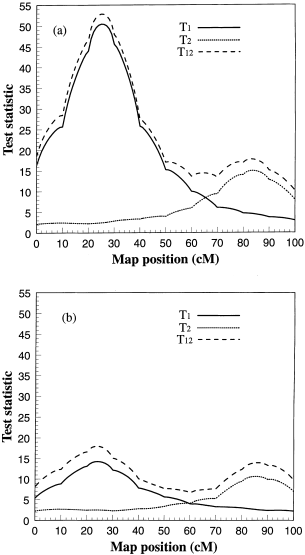
Finally, selective genotyping has increased the score of the test statistic up to threefold (see the last column of Table 2). MULTIPLE TRAIT QTL MAPPING In the second simulation study, we

investigated QTL mapping for two correlated traits under selective genotyping. The marker map remains the same as previously described. The first trait is controlled by one QTL at the same

location (25 cM) with the same effect as described in the previous experiment, i.e. _a_1=0.229 and _d_1= 0.162. The second trait is controlled by a QTL located at 85 cM with identical

effects, i.e. _a_2=0.229 and _d_2=0.162. The residual variances were set at σ21=σ22=1 and the residual covariance set at σ12=0.5. The selection criterion was _I__j_=_c_1_y__j_1 + _c_2_y__j_2

where _c_1=1 and _c_2=0, i.e. only the first trait was selected. A total of 2500 individuals were measured for phenotype, but 250 (10%) were selectively genotyped. The simulation was

replicated 50 times. Figure 1 gives the average likelihood ratio test statistic profiles under selective genotyping (10%). The solid (_T_1), dotted (_T_2) and dashed (_T_12) lines represent

the likelihood-ratio test statistic profiles for the first trait, the second trait and both traits (joint test), respectively. Note that the likelihood-ratio test statistic profiles

(functions of the _F_-test statistics) are used here. They are defined as: and where _σ^_2Ω is the estimated residual variance under model Ω which defines the linear model by the set of

parameters included in the model: We used _T_ instead of λ to depict the test statistic profiles because _T_ approximates a χ2_q_ distribution and thus bears the additive property, i.e.

_T_12=_T_1 + _T_2. Although the two traits have an identical genetic variance, the first trait has a substantially higher test statistic profile than the second one because the first trait

is directly selected for genotyping. As a comparison, we repeated the simulation under random selection, i.e. we generated 250 individuals and genotyped all of them (100%) for mapping. The

corresponding test statistic profiles are given in Fig. 1(b). Compared with random selection (Fig. 1b), the increase in the test statistic profile for the first trait (Fig. 1a) is obvious. A

slight increase in the test statistic profile for the second trait is also observed because of its correlation to the first trait. POWER UNDER SELECTIVE GENOTYPING As reported in this

section, we first calculated the predicted powers under various proportions of genotyped individuals using the theoretical formula given in eqn (18). We then conducted simulation experiments

to verify our theoretical prediction. The effects of the QTL were again set at _a_=0.229 and _d_=0.162. The number of individuals genotyped remained at _n_=100. We varied the total number

of individuals measured (_N_) to control the proportions selected for genotyping (see column 2 of Table 3). Because the population mean was set at μ = 0, the truncation points are

symmetrical, and thus _t_2=−_t_1, where the values of _t_1 were found by trial and error so that the theoretical proportions selected equal the predetermined proportions (see column 3 of

Table 3). The values of the noncentrality parameter are listed in column 4 of Table 3. The critical value for testing the hypothesis at a Type I error rate of α=0.05 is _F_−1(0.95 : 2, 97,

0)=3.09, which was used to calculate the theoretical powers (listed in column 5 of Table 3). We then simulated 1000 samples under each level of proportion and conducted QTL analysis for each

sampled data set. The empirical power under each setting was calculated as the proportion of the samples that have the _F-_like test statistic greater than 3.09. These empirical powers,

given in the last column of the table, are fairly close to the corresponding theoretical predictions. DISCUSSION When the phenotypic values of ungenotyped individuals are included in the

data analysis, standard methods with proper handling of missing markers are used (Lander & Botstein, 1989; Muranty & Goffinet, 1997a,b; Henshall & Goddard, 1999; Johnson et al.,

1999). A problem occurs if the number of ungenotyped individuals is large because of the increased computational burden; for example, if 10% of the test population is genotyped, to genotype

250 individuals, one needs to measure an additional 2250 individuals for their phenotypes. The total sample size will be 2500. Because the 2250 ungenotyped individuals contribute very little

to linkage analysis but serve as bias correctors, their phenotypic values do not have to be included in the analysis. These individuals, however, do contribute to the estimation of the

residual variance. The estimate of the residual variance usually has very small estimation error. When the number of individuals genotyped is small, however, the residual variance estimate

from only the genotyped individuals may not be sufficiently accurate. In this case, it is important to include the ungenotyped individuals. The methods described above (e.g. Muranty &

Goffinet, 1997a,bJohnson et al., 1999) are not the only ways to include the ungenotyped individuals. An alternative way is to ignore completely the genetic effects for the ungenotyped

individuals, partition the residual variance of an ungenotyped individual into a genetic and a pure environmental component, and use a mixed-model approach. This can be accomplished via the

following maximum likelihood analysis. Define the model for an ungenotyped individual by _y__j_=μ + _r__j_ for _j_=_n_ + 1, …, _N_, where _r__j_ is the residual effect with an N(0, σ2G + σ2)

distribution and σ2G=_a_2/2 + _d_2, as defined previously. The probability density of _y__j_ for the ungenotyped individual will be: The likelihood function including all individuals will

be: Note that ungenotyped individuals do not contribute to the estimation of B except μ, but they are used to estimate σ2G + σ2. The MLE may be directly searched or obtained via an EM

algorithm. In either way, the speed of convergence may be faster than the methods that treat X_j_ as missing values because there is no need to update _p_(X_j_) for an ungenotyped

individual. Further investigation is required to explore the properties of this alternative approach. It is not hard to imagine that ungenotyped individuals may not have a full measurement

of phenotypic values. This may occur, for example, in QTL mapping for the trait of flowering time. An investigator may choose to visit the field for the first few days when the population of

plants begins to flower and the last few days when the population approaches the end of the flowering season. In this case, plants that flower in the middle of the season may not have a

record of phenotype. Another example comes from multiple trait analysis in forest trees. One may decide to select early growth rate for QTL mapping, but later the investigator may want to

map QTLs for later growth rate as well. If selection is on the early trait, because of limited space, the investigator may not keep the culled individuals in the field. Then the final

population would be a selected population with regard to the later growth rate. The maximum likelihood analysis proposed in this study is the proper tool for handling such centrally

truncated data. It is undesirable to use only one tail of the trait distribution to carry out QTL mapping because the total variance of the trait is artificially deflated. However, if the

data happen to be single-tail truncated for some technical reasons, the proposed method can readily be applied for correcting the bias. A typical example of single-tail truncation can be

seen in artificial selection of plant and animal breeding. Another example may come from longitudinal data analysis where the phenotypic value of an individual depends on it longevity. Only

surviving individuals have a complete measurement of phenotype, whereas individuals not surviving only have partial information; for example, the yearly egg production of a chicken strongly

depends on the viability of the chicken. If a chicken dies in the middle of the year, we do not know the phenotypic record of her yearly production, but we do know that her yearly egg

production is greater than the current production in her record at the time when she dies. An unbiased analysis must be performed by taking into account these partial records. For

multiple-trait analysis, selective genotyping has been a problem because if all traits are deemed to be important to the researcher, which traits should be selected? The selection index

approach of Muranty & Goffinet (1997b) is a compromise between the traits. Because the selection criterion now becomes a single ‘trait’, it is easy to apply in practice. Lin &

Ritland (1997) suggested that an individual should be genotyped if at least one of _m_ traits exhibits the extreme value. Under this selection regime, different individuals seem to have

different criteria of selection; for example, if individual _j_ is selected because its _k_th phenotypic value is first observed as being extreme, then the criterion for _j_ is (_y__jk_ ≤

_t_1_k_) ⋃ (_y__jk_ ≥ _t_2_k_). On the other hand, if individual _i_ is selected because its _l_th phenotypic value is first observed as being extreme, then the criterion for _i_ is (_y__il_

≤ _t_1_l_) ⋃ (_y__il_ ≥ _t_2_l_). In both the index selection and the method of Lin & Ritland (1997), the selection criterion of each individual is a single trait (one-dimensional

selection), and thus the proposed method will apply. Another selection regime may be the so-called independent culling level selection where an individual will not be genotyped if any one of

the _m_ phenotypic values fails to reach the extreme. This selection regime is perhaps more rigorous than the previous two methods, but it is hard to programme because it is a multiple

dimensional selection (requiring multiple integration). Further study may be necessary to compare different selection regimes. Nonetheless, when phenotypic values of ungenotyped individuals

are included, methods of selection will be irrelevant to the statistical issue. Once selection is carried out on the phenotypic value of one trait (primary trait), QTL mapping for a highly

correlated trait (secondary trait) will also benefit. However, if the two traits are not correlated, the effective sample size in terms of the secondary trait will be comparable to a

_random_ sample of _n_, where _n_ is the number of genotyped individuals. Therefore, one should be cautious about the power of QTL mapping for traits less correlated to a highly selected

primary trait. An advantage of the logistic regression of Henshall & Goddard (1999) is that selection does not bias estimates of QTL effects, irrespective of whether phenotypic values of

ungenotyped individuals are included in the data analysis. This is because the roles of marker genotypes and the phenotypes in the likelihood function have been altered, just like the

discordant sib-pair mapping of Risch & Zhang (1995). Further investigation on the logistic regression, however, shows that selective genotyping can alter the estimation of the QTL

effect. The equivalence between logistic regression and the maximum likelihood holds only approximately when the effect of a QTL is small. This can be shown by looking at the posterior

probability of a QTL genotype given the phenotypic value of individual _j_: where _p_(X_j_) is the prior probability of the QTL genotype, independent of marker information, and

_g_(_y__j_|X_j_)=[_f_(_y__j_|X_j_)]/{Φ(τ1|X_j_)+[1 − Φ(τ2|X_j_)]}. However, the logistic regression model uses r ( x j ) = [ p ( x j ) f ( y j | x j ) ] / [ Σ x j ∈ S p ( x j ) f ( y j | x j

) ] , i.e. the term Φ(τ1|X_j_)+[1 − Φ(τ2|X_j_)] in the denominator of _g_(_y__j_|X_j_) has vanished. The exact maximum likelihood function should be built using _p_*(X_j_) instead of

_r_(X_j_). However, using _r_(X_j_) may still be justifiable because: (i) when the size of the QTL is small, Φ(τ1|X_j_) + [1 − Φ(τ2|X_j_)] can be considered as a constant across different

genotypes so that the corresponding terms in the numerator and denominator cancel each other out, leading to _p_*(X_j_) ≈ _r_(X_j_); and (ii) _r_(X_j_) is much easier to handle than

_p_*(X_j_) in the maximum likelihood analysis. In addition to the approximate nature of the logistic regression, there are two unsolved problems: (a) modification is required to map a QTL in

an F2 population; and (b) an exact interval mapping has not been available. An approximate interval mapping was accomplished via interpolation (Henshall & Goddard, 1999). Solving for

the first problem requires a multicategorical response model, e.g. models for nominal or ordinal responses (Fahrmeir & Tutz, 1994). The second problem involves missing QTL genotypes and

may be solved using the EM or MCMC algorithm of C. Vogl & S. Xu (unpublished results) for mapping viability loci. Quantitative trait loci mapping is usually performed after a marker map

is fully developed. If the trait under selection has a strong genetic component, selective genotyping can also cause distortion of the inferred marker map from the true one. The distortion

is reflected by the change in both the marker order and the distances between markers. Because the severity of marker map distortion depends on the sizes and locations of QTLs, marker

mapping and QTL mapping should be carried out concurrently under selective genotyping. One can apply the general idea of EM to concurrent mapping. To do this, one first maps QTLs under the

assumption that the marker map is known without error, and then corrects the marker map by taking into account the distortion caused by selective genotyping under the assumption that the

sizes and locations of QTLs are known. This completes one cycle of iteration, and the iteration should continue until a criterion of convergence is reached. The problem can be very

complicated, especially when the marker order is allowed to change. Many theoretical and practical problems may exist in concurrent mapping, and further investigation is deemed necessary.

Maximization of the likelihood function is not an easy task. Special algorithms and computer programs are required. We developed an EM algorithm that appears to be a simple modification of

the existing EM algorithm for standard interval mapping. As a result, it can be readily incorporated into a standard QTL mapping software, e.g. MAPMAKER (Lander & Botstein, 1989). One

caveat about the EM algorithm is that when the selection intensity is too high, the EM algorithm may take a very large number of iterations to converge and sometime may not converge at all.

This is not a problem of the EM algorithm itself, rather, it is caused by numerical overflow when the bias adjustment of the residual variance is conducted. Recall that we added an

additional term in eqn (8), σ2[(τ1|X_j_)φ(τ1|X_j_) − (τ2|X_j_)φ(τ2|X_j_)]/[1 + Φ(τ1|X_j_) − Φ(τ2|X_j_)], to the standard EM estimation of the residual variance. When the selection intensity

is high, this term can be numerically unstable. Proper handling of this numerical overflow is required which is, unfortunately, beyond our technical ability. We found that when the

proportion selected is 40% or more, the problem rarely happens. In our simulation studies, when numerical overflow occurred, the EM algorithm was replaced by the simplex algorithm (Nelder

& Mead, 1965) for direct search of MLEs. The simplex method is usually slower than the EM algorithm, but it can handle highly selected data. Another caveat is the sensitivity of the

proposed method to departure from normality. Because the likelihood function involves Φ(τ), in addition to φ(τ), we anticipate that the method is more sensitive to deviation from normality

than the methods using also the ungenotyped individuals. In conclusion, we developed an exact maximum likelihood approach to map QTLs under selective genotyping using phenotypic values of

genotyped individuals only. Compared with the full data analysis (using all phenotypic values), the proposed method performs well: the average test statistic is slightly lower; estimates of

QTL parameters are almost identical; and the estimate of residual variance is subject to a relatively large error. The slightly lower test statistic value may be caused by the relatively

large increase in the estimation error of the residual variance. A general recommendation is that whenever full data analysis is possible, the full maximum likelihood analysis should be

performed. If it is impossible or difficult to analyse the full data, e.g. the sample size is too large, the phenotypic values of ungenotyped individuals are missing or composite interval

mapping is to be performed, then the proposed method should be applied with the understanding that there is little to lose. REFERENCES * Cohen, A. C. (1991). _Truncated and Censored Samples

— Theory and Applications_. Marcel Dekker, New York. Book  Google Scholar  * Darvasi, A. and Soller, M. (1992). Selective genotyping for determination of linkage between a marker locus and a

quantitative trait locus. _Theor Appl Genet_, 85: 353–359. Article  CAS  PubMed  Google Scholar  * Fahrmeir, L. and Tutz, G. (1994). _Multivariate Statistical Modelling Based on Generalized

Linear Models_. Springer-Verlag, New York, NY. Book  Google Scholar  * Graybill, F. A. (1976). _Theory and Application of the Linear Model_. Duxbury Press, North Scituate, MA. Google

Scholar  * Groover, A., Devey, M., Fiddler, T., Lee, J., Megraw, R., Mitchell-Olds, T. _et al_ (1994). Identification of quantitative trait loci influencing wood specific gravity in an

outbred pedigree of loblolly pine. _Genetics_ 138: 1293–1300. CAS  PubMed  PubMed Central  Google Scholar  * Henshall, J. M. and Goddard, M. E. (1999). Multiple-trait mapping of quantitative

trait loci after selective genotyping using logistic regression. _Genetics_ 151: 885–894. CAS  PubMed  PubMed Central  Google Scholar  * Jansen, R. C. and Stam, P. (1994). High resolution

of quantitative traits into multiple loci via interval mapping. _Genetics_ 136: 1447–1455. CAS  PubMed  PubMed Central  Google Scholar  * Jiang, C. and Zeng, Z. B. (1995). Multiple trait

analysis of genetic mapping for quantitative trait loci. _Genetics_ 140: 1111–1127. CAS  PubMed  PubMed Central  Google Scholar  * Johnson, D. L., van Jansen, R. C. and Arendonk, A. M.

(1999). Mapping quantitative trait loci in a selectively genotyped outbred population using a mixture model approach. _Genet Res_, 73: 75–83. Article  Google Scholar  * Lander, E. S. and

Botstein, D. (1989). Mapping Mendelian factors underlying quantitative traits using RFLP linkage maps. _Genetics_ 121: 185–199. CAS  PubMed  PubMed Central  Google Scholar  * Lin, J. Z. and

Ritland, K. (1997). Quantitative trait loci differentiating the outbreeding _Mimulus guttatus_ from the inbreeding _M. platycalyx_. _Genetics_ 146: 1115–1121. CAS  PubMed  PubMed Central 

Google Scholar  * Muranty, H. (1996). Power of tests for quantitative trait loci detection using full-sib families in different schemes. _Heredity_ 76: 156–165. Article  Google Scholar  *

Muranty, H. and Goffinet, B. (1997a). Selective genotyping for location and estimation of the effect of a quantitative trait locus. _Biometrics_ 53: 629–643. Article  Google Scholar  *

Muranty, H. and Goffinet, B. (1997b). Multitrait and multipopulation QTL search using selective genotyping. _Genet Res_, 70: 259–265. Article  Google Scholar  * Nelder, J. A. and Mead, R.

(1965). A simplex method for function minimization. _Comput J_, 7: 308–313. Article  Google Scholar  * Risch, N. and Zhang, H. (1995). Extreme discordant sib pairs for mapping quantitative

trait loci in humans. _Science_ 268: 1584–1589. Article  CAS  PubMed  Google Scholar  * Soller, M. and Brody, T. (1976). On the power of experimental designs for the detection of linkage

between marker loci and quantitative trait loci in crosses between inbred lines. _Theor Appl Genet_, 47: 35–39. Article  CAS  PubMed  Google Scholar  * Zeng, Z. B. (1994). Precision mapping

of quantitative trait loci. _Genetics_ 136: 1457–1468. CAS  PubMed  PubMed Central  Google Scholar  Download references ACKNOWLEDGEMENTS Many thanks are due to Drs W. M. Muir and O.

Savolainen for their encouragement and support on the project. We thank Drs D. Gessler, J. Lin, R. Whitkus and M. Sillanpaa for their helpful comments on an earlier version of the

manuscript. We would also like to thank two anonymous reviewers for their criticisms and comments which have greatly improved the presentation of the manuscript. This research was supported

by the National Institutes of Health Grant GM55321 and the USDA National Research Initiative Competitive Grants Program 97–35205–5075 to S.X. AUTHOR INFORMATION Author notes * Claus Vogl

Present address: Department of Botany and Plant Sciences, University of California, Riverside, CA 92521, U.S.A. AUTHORS AND AFFILIATIONS * Department of Botany and Plant Sciences, University

of California, Riverside, 92521, CA, USA Shizhong Xu * Department of Biology, University of Oulu, PO Box 3000, Oulu, FIN-90401, Finland Claus Vogl Authors * Shizhong Xu View author

publications You can also search for this author inPubMed Google Scholar * Claus Vogl View author publications You can also search for this author inPubMed Google Scholar CORRESPONDING

AUTHOR Correspondence to Shizhong Xu. APPENDIX DERIVATION OF THE EM ALGORITHM FOR SINGLE-TRAIT ANALYSIS APPENDIX DERIVATION OF THE EM ALGORITHM FOR SINGLE-TRAIT ANALYSIS First, let us define

the log likelihood function by: The MLEs of B and σ2 are obtained by solving ∂_l_/∂B=0 and ∂_l_/∂σ2=0 simultaneously. Derivation of ∂l/∂B where In the above equation, the truncation points

have been standardized, i.e. τ1=(_t_1 − X_j_B)/σ and τ2=(_t_2 − X_j_B)/σ, where _t_1 and _t_2 are the truncation points in the original scale. Note that: Hence, Define

_p_*(X_j_)=[_p_(X_j_)_g_(_y__j_|X_j_)]/[ ∑ x j ε_S__ p_(X_j_)_g_(_y__j_|X_j_)] as the posterior distribution of X_j_. We now have: Solving for ∂_l_/∂B=0, we have: Derivation of ∂l/∂σ2 where

Note that Therefore, Finally, we have Solving for ∂_l_/∂σ2=0, we obtain RIGHTS AND PERMISSIONS Reprints and permissions ABOUT THIS ARTICLE CITE THIS ARTICLE Xu, S., Vogl, C. Maximum

likelihood analysis of quantitative trait loci under selective genotyping. _Heredity_ 84, 525–537 (2000). https://doi.org/10.1046/j.1365-2540.2000.00653.x Download citation * Received: 22

June 1999 * Accepted: 13 October 1999 * Published: 01 May 2000 * Issue Date: 01 May 2000 * DOI: https://doi.org/10.1046/j.1365-2540.2000.00653.x SHARE THIS ARTICLE Anyone you share the

following link with will be able to read this content: Get shareable link Sorry, a shareable link is not currently available for this article. Copy to clipboard Provided by the Springer

Nature SharedIt content-sharing initiative KEYWORDS * EM algorithm * QTL mapping * simplex algorithm * truncated selection